Data Mining Data Lecture Notes for Chapter 2

Data Mining: Data Lecture Notes for Chapter 2 Introduction to Data Mining by Tan, Steinbach, Kumar Revised by QY © Tan, Steinbach, Kumar Introduction to Data Mining 4/18/2004 1

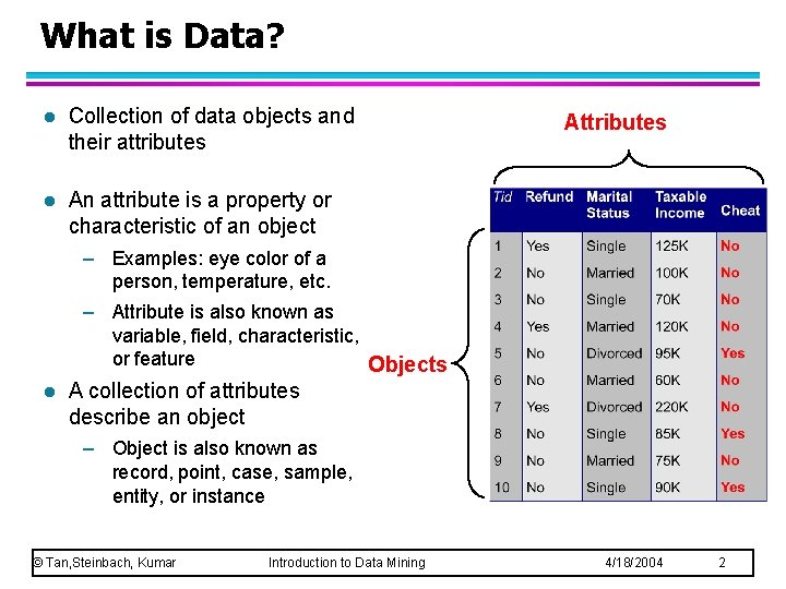
What is Data? l Collection of data objects and their attributes l An attribute is a property or characteristic of an object Attributes – Examples: eye color of a person, temperature, etc. – Attribute is also known as variable, field, characteristic, or feature Objects l A collection of attributes describe an object – Object is also known as record, point, case, sample, entity, or instance © Tan, Steinbach, Kumar Introduction to Data Mining 4/18/2004 2

Attribute Values l Attribute values are numbers or symbols assigned to an attribute – E. g. ‘Student Name’=‘John’ – Attributes are also called ‘variables’, or ‘features’ – Attribute values are also called ‘values’, or ‘featurevalues’ l Designing Attributes for a data set requires domain knowledge – Always have an objective in mind (e. g. , what is the class attribute? ) – Design a ‘movie’ data set for a movie dataset? u. What © Tan, Steinbach, Kumar is domain knowledge? Introduction to Data Mining 4/18/2004 3

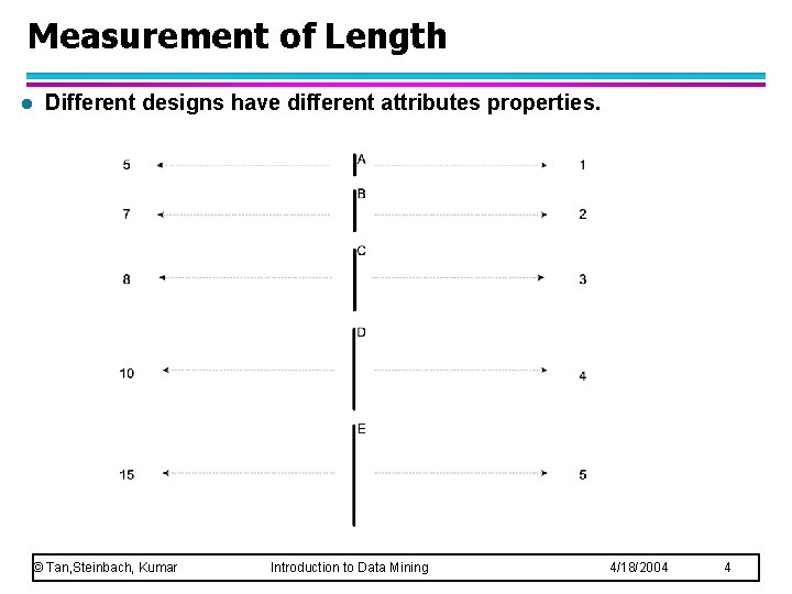
Measurement of Length l Different designs have different attributes properties. © Tan, Steinbach, Kumar Introduction to Data Mining 4/18/2004 4

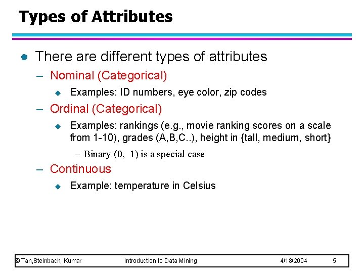
Types of Attributes l There are different types of attributes – Nominal (Categorical) u Examples: ID numbers, eye color, zip codes – Ordinal (Categorical) u Examples: rankings (e. g. , movie ranking scores on a scale from 1 -10), grades (A, B, C. . ), height in {tall, medium, short} – Binary (0, 1) is a special case – Continuous u Example: temperature in Celsius © Tan, Steinbach, Kumar Introduction to Data Mining 4/18/2004 5

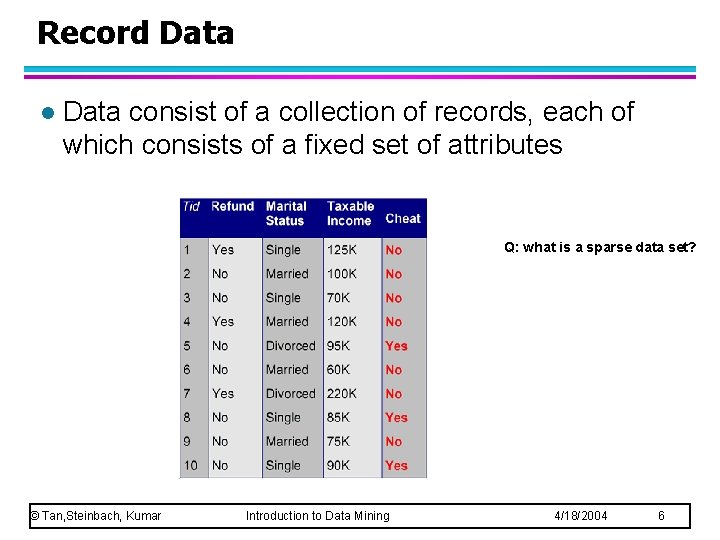
Record Data l Data consist of a collection of records, each of which consists of a fixed set of attributes Q: what is a sparse data set? © Tan, Steinbach, Kumar Introduction to Data Mining 4/18/2004 6

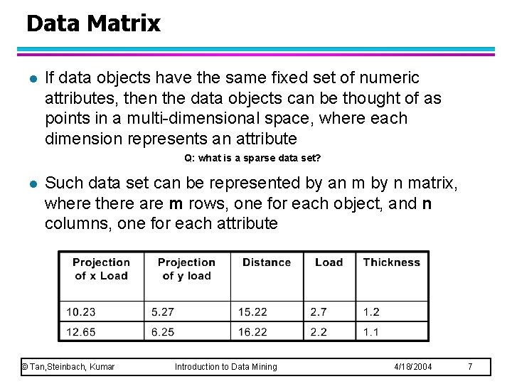
Data Matrix l If data objects have the same fixed set of numeric attributes, then the data objects can be thought of as points in a multi-dimensional space, where each dimension represents an attribute Q: what is a sparse data set? l Such data set can be represented by an m by n matrix, where there are m rows, one for each object, and n columns, one for each attribute © Tan, Steinbach, Kumar Introduction to Data Mining 4/18/2004 7

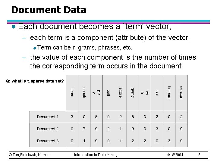
Document Data l Each document becomes a `term' vector, – each term is a component (attribute) of the vector, u. Term can be n-grams, phrases, etc. – the value of each component is the number of times the corresponding term occurs in the document. Q: what is a sparse data set? © Tan, Steinbach, Kumar Introduction to Data Mining 4/18/2004 8

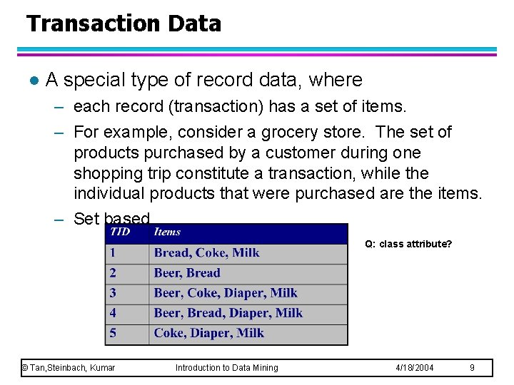
Transaction Data l A special type of record data, where – each record (transaction) has a set of items. – For example, consider a grocery store. The set of products purchased by a customer during one shopping trip constitute a transaction, while the individual products that were purchased are the items. – Set based Q: class attribute? © Tan, Steinbach, Kumar Introduction to Data Mining 4/18/2004 9

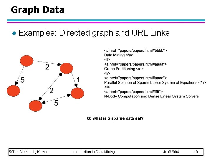
Graph Data l Examples: Directed graph and URL Links Q: what is a sparse data set? © Tan, Steinbach, Kumar Introduction to Data Mining 4/18/2004 10

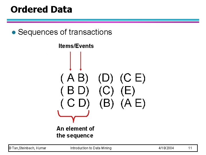
Ordered Data l Sequences of transactions Items/Events An element of the sequence © Tan, Steinbach, Kumar Introduction to Data Mining 4/18/2004 11

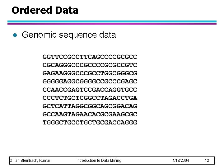
Ordered Data l Genomic sequence data © Tan, Steinbach, Kumar Introduction to Data Mining 4/18/2004 12

Data Quality What kinds of data quality problems? l How can we detect problems with the data? l What can we do about these problems? l l Examples of data quality problems: – Noise and outliers – missing values – duplicated data © Tan, Steinbach, Kumar Introduction to Data Mining 4/18/2004 13

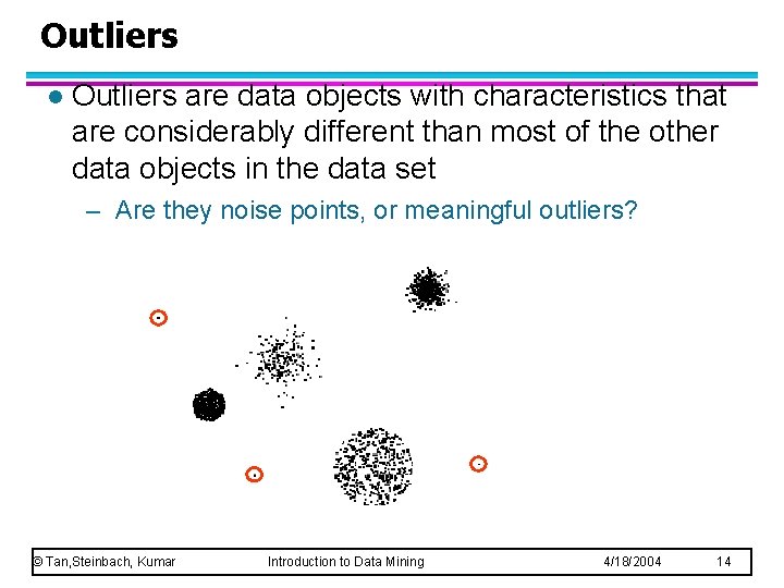
Outliers l Outliers are data objects with characteristics that are considerably different than most of the other data objects in the data set – Are they noise points, or meaningful outliers? © Tan, Steinbach, Kumar Introduction to Data Mining 4/18/2004 14

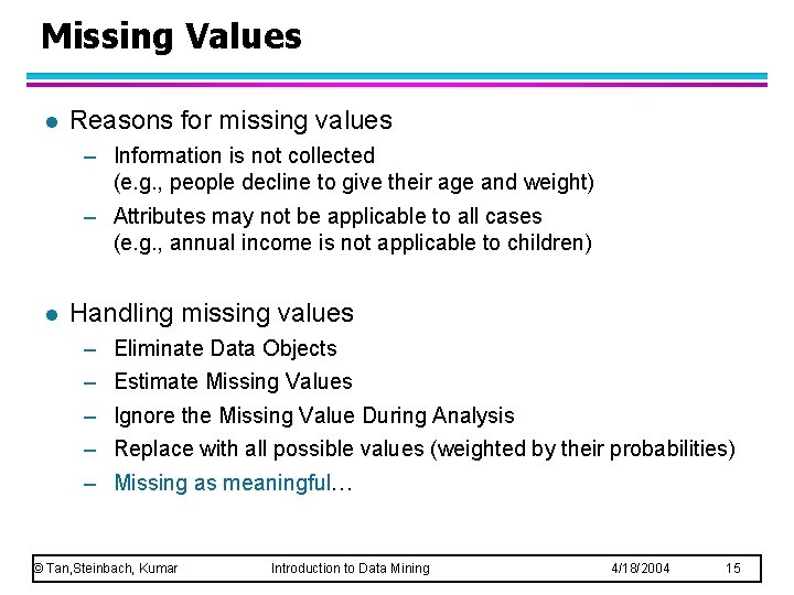
Missing Values l Reasons for missing values – Information is not collected (e. g. , people decline to give their age and weight) – Attributes may not be applicable to all cases (e. g. , annual income is not applicable to children) l Handling missing values – – – Eliminate Data Objects Estimate Missing Values Ignore the Missing Value During Analysis Replace with all possible values (weighted by their probabilities) Missing as meaningful… © Tan, Steinbach, Kumar Introduction to Data Mining 4/18/2004 15

Data Preprocessing Aggregation and Noise Removal l Sampling l Dimensionality Reduction l Feature subset selection l Feature creation and transformation l Discretization l l Q: How much % of the data mining process is data preprocessing? © Tan, Steinbach, Kumar Introduction to Data Mining 4/18/2004 16

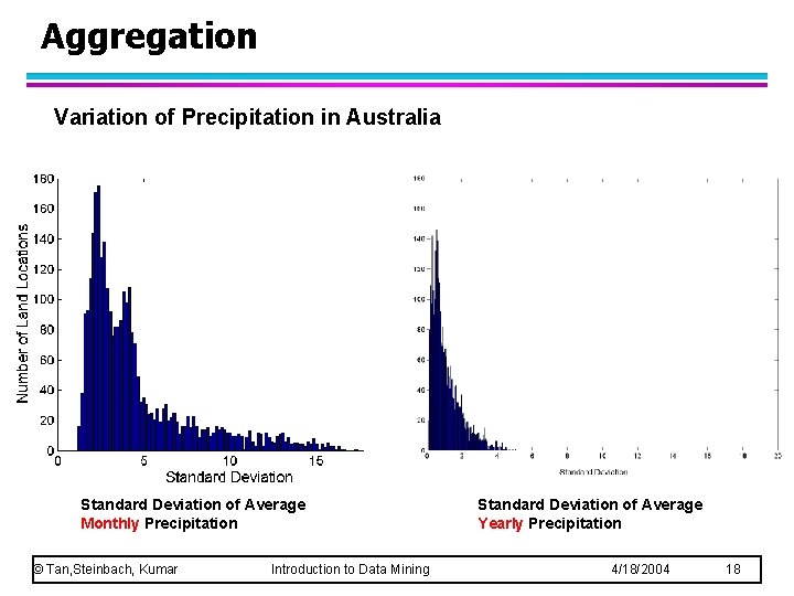
Aggregation l Combining two or more attributes (or objects) into a single attribute (or object) l Purpose – Data reduction u Reduce the number of attributes or objects – Change of scale u Cities aggregated into regions, states, countries, etc – De-noise: more “stable” data u Aggregated data tends to have less variability © Tan, Steinbach, Kumar Introduction to Data Mining 4/18/2004 17

Aggregation Variation of Precipitation in Australia Standard Deviation of Average Monthly Precipitation © Tan, Steinbach, Kumar Introduction to Data Mining Standard Deviation of Average Yearly Precipitation 4/18/2004 18

Sampling l Sampling is the main technique employed for data selection. – It is often used for both the preliminary investigation of the data and the final data analysis. l Reasons: – too expensive or time consuming to obtain or to process the data. © Tan, Steinbach, Kumar Introduction to Data Mining 4/18/2004 19

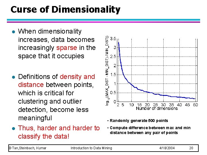
Curse of Dimensionality l When dimensionality increases, data becomes increasingly sparse in the space that it occupies l Definitions of density and distance between points, which is critical for clustering and outlier detection, become less meaningful Thus, harder and harder to classify the data! l © Tan, Steinbach, Kumar • Randomly generate 500 points • Compute difference between max and min distance between any pair of points Introduction to Data Mining 4/18/2004 20

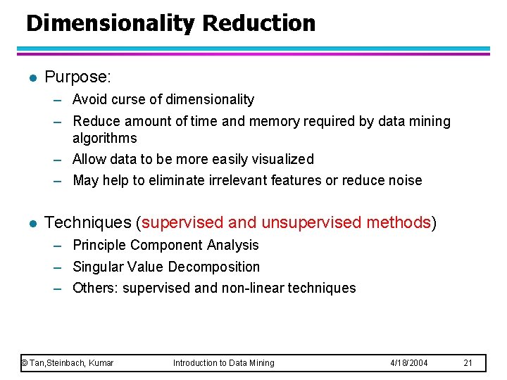
Dimensionality Reduction l Purpose: – Avoid curse of dimensionality – Reduce amount of time and memory required by data mining algorithms – Allow data to be more easily visualized – May help to eliminate irrelevant features or reduce noise l Techniques (supervised and unsupervised methods) – Principle Component Analysis – Singular Value Decomposition – Others: supervised and non-linear techniques © Tan, Steinbach, Kumar Introduction to Data Mining 4/18/2004 21

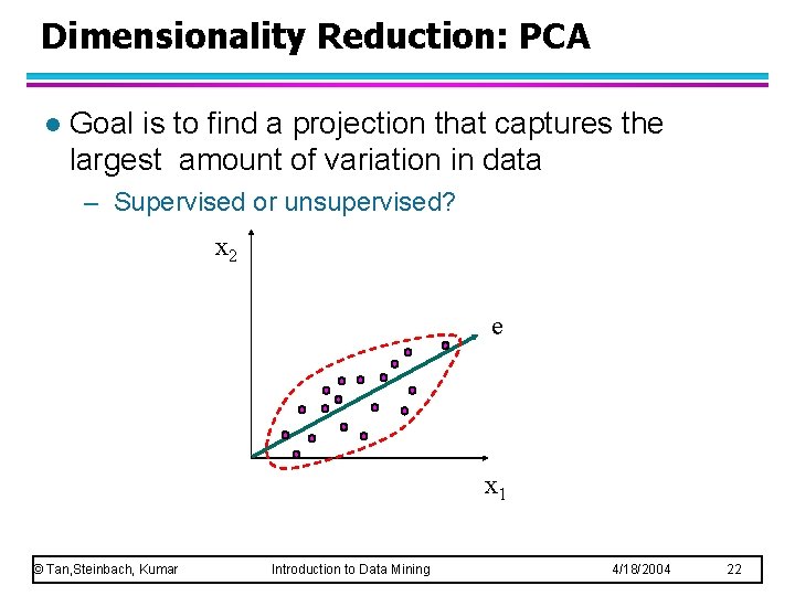
Dimensionality Reduction: PCA l Goal is to find a projection that captures the largest amount of variation in data – Supervised or unsupervised? x 2 e x 1 © Tan, Steinbach, Kumar Introduction to Data Mining 4/18/2004 22

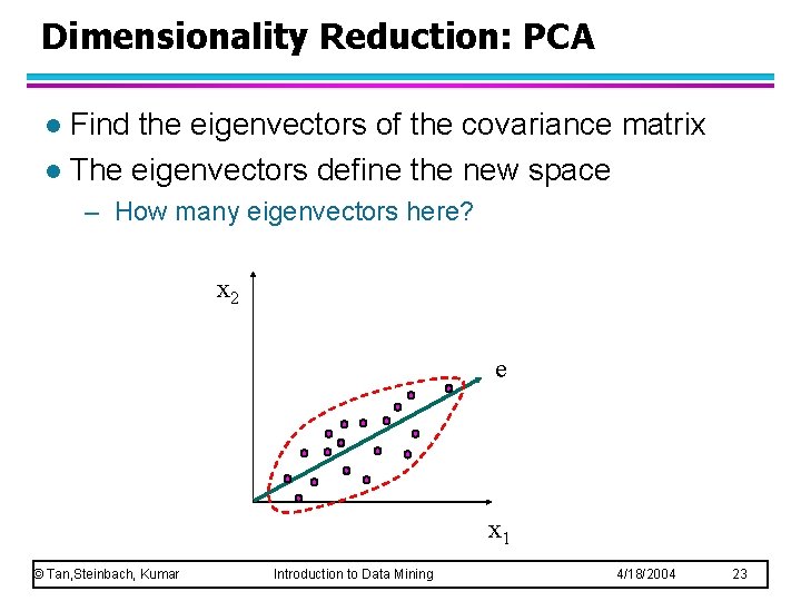
Dimensionality Reduction: PCA Find the eigenvectors of the covariance matrix l The eigenvectors define the new space l – How many eigenvectors here? x 2 e x 1 © Tan, Steinbach, Kumar Introduction to Data Mining 4/18/2004 23

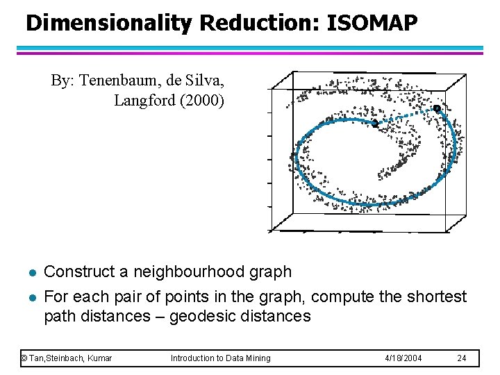
Dimensionality Reduction: ISOMAP By: Tenenbaum, de Silva, Langford (2000) l l Construct a neighbourhood graph For each pair of points in the graph, compute the shortest path distances – geodesic distances © Tan, Steinbach, Kumar Introduction to Data Mining 4/18/2004 24

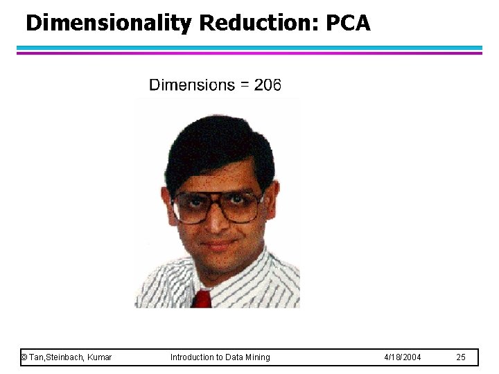
Dimensionality Reduction: PCA © Tan, Steinbach, Kumar Introduction to Data Mining 4/18/2004 25

Question l What is the difference between sampling and dimensionality reduction? – Thining vs. shortening of data © Tan, Steinbach, Kumar Introduction to Data Mining 4/18/2004 26

Discretization l Three types of attributes: – Nominal — values from an unordered set u. Example: attribute “outlook” from weather data – Values: “sunny”, ”overcast”, and “rainy” – Ordinal — values from an ordered set u. Example: attribute “temperature” in weather data – Values: “hot” > “mild” > “cool” – Continuous — real numbers l Discretization: – – divide the range of a continuous attribute into intervals Some classification algorithms only accept categorical attributes. Reduce data size by discretization Supervised (entropy) vs. Unsupervised (binning) © Tan, Steinbach, Kumar Introduction to Data Mining 4/18/2004 27

Simple Discretization Methods: Binning l Equal-width (distance) partitioning: – It divides the range into N intervals of equal size: uniform grid – if A and B are the lowest and highest values of the attribute, the width of intervals will be: W = (B –A)/N. u. The most straightforward u. But outliers may dominate presentation: Skewed data is not handled well. l Equal-depth (frequency) partitioning: – It divides the range into N intervals, each containing approximately same number of samples – Good data scaling – Managing categorical attributes can be tricky. © Tan, Steinbach, Kumar Introduction to Data Mining 4/18/2004 28

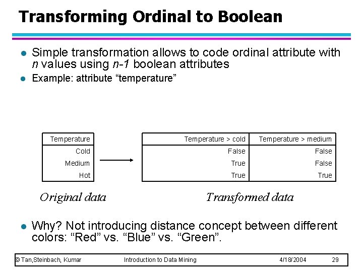
Transforming Ordinal to Boolean l Simple transformation allows to code ordinal attribute with n values using n-1 boolean attributes l Example: attribute “temperature” Temperature > cold Temperature > medium Cold False Medium True False Hot True Original data l Transformed data Why? Not introducing distance concept between different colors: “Red” vs. “Blue” vs. “Green”. © Tan, Steinbach, Kumar Introduction to Data Mining 4/18/2004 29

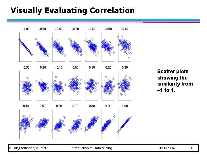
Visually Evaluating Correlation Scatter plots showing the similarity from – 1 to 1. © Tan, Steinbach, Kumar Introduction to Data Mining 4/18/2004 30