Data Mining Data Lecture Notes for Chapter 2

Data Mining: Data Lecture Notes for Chapter 2 1

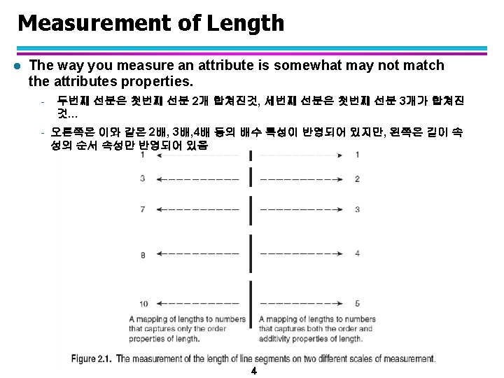
2. 1 Types of Data - What is Data? l Collection of data objects and their attributes l An attribute is a property or characteristic of an object Attributes – Examples: eye color of a person, temperature, etc. – Attribute is also known as variable, field, characteristic, or feature Objects l A collection of attributes describe an object – Object is also known as record, point, case, sample, entity, or instance 2

Attribute Values l Attribute values are numbers or symbols assigned to an attribute l Distinction between attributes and attribute values – Same attribute can be mapped to different attribute values u Example: height can be measured in feet or meters – Different attributes can be mapped to the same set of values u Example: Attribute values for ID and age are integers u But properties of attribute values can be different – ID has no limit but age has a maximum and minimum value 3

Types of Attributes l There are different types of attributes – Nominal(명목형) u Examples: ID numbers, eye color, zip codes – Ordinal(서열형) u Examples: rankings (e. g. , taste of potato chips on a scale from 1 -10), grades, height in {tall, medium, short} – Interval(구간형) u Examples: calendar dates, temperatures in Celsius or Fahrenheit. – Ratio(비율형) u Examples: temperature in Kelvin, length, time, counts 5

Properties of Attribute Values l The type of an attribute depends on which of the following properties it possesses: – Distinctness(유일성): = – Order(순서): < > – Addition(덧셈): + - – Multiplication(곱셈): * / – Nominal attribute(명목형): distinctness – Ordinal attribute(서열형): distinctness & order – Interval attribute(구간형): distinctness, order & addition – Ratio attribute(비율형): all 4 properties 6

Attribute Type Description Examples Operations Nominal The values of a nominal attribute are just different names, i. e. , nominal attributes provide only enough information to distinguish one object from another. (=, ) zip codes, employee ID numbers, eye color, sex: {male, female} mode, entropy, contingency correlation, 2 test hardness of minerals, {good, better, best}, grades, street numbers Median(중간값), percentiles, rank correlation, run tests, sign tests calendar dates, temperature in Celsius or Fahrenheit mean, standard deviation, Pearson's correlation, t and F tests temperature in Kelvin, monetary quantities, counts, age, mass, length, electrical current geometric mean, harmonic mean, percent variation(퍼 센트 편차) (명목형은 단순히 서로 다른 이름뿐 서로 구별 정보만 제공) Ordinal The values of an ordinal attribute provide enough information to order objects. (<, >) (서열형은 서로 순서를 정하는데 필요한 정보 제공) Interval For interval attributes, the differences between values are meaningful, i. e. , a unit of measurement exists. (+, - ) (구간형은 값들 사이의 차이가 의미가 있 음) Ratio For ratio variables, both differences and ratios are meaningful. (*, /) (비율형은 차이와 비율이 모두 의미가 있 음)

< 속성 수준을 정의한 변환예 > Attribute Level Transformation Nominal Any permutation of values (순서 변환: 순열) If all employee ID numbers were reassigned, would it make any difference? Ordinal An order preserving change of values, i. e. , new_value = f(old_value) where f is a monotonic function. (값의 순서 보존형 변환) An attribute encompassing the notion of good, better best can be represented equally well by the values {1, 2, 3} or by { 0. 5, 1, 10}. Interval new_value =a * old_value + b where a and b are constants (새값 = a*예전값 + b) Thus, the Fahrenheit and Celsius temperature scales differ in terms of where their zero value is and the size of a unit (degree). new_value = a * old_value (새값 = a * 예전값) Length can be measured in meters or feet. Ratio Comments

Discrete and Continuous Attributes l Discrete Attribute – Has only a finite or countably infinite set of values – Examples: zip codes, counts, or the set of words in a collection of documents – Often represented as integer variables. – Note: binary attributes are a special case of discrete attributes l Continuous Attribute – Has real numbers as attribute values – Examples: temperature, height, or weight. – Practically, real values can only be measured and represented using a finite number of digits. – Continuous attributes are typically represented as floating-point variables. 9

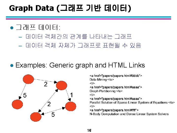
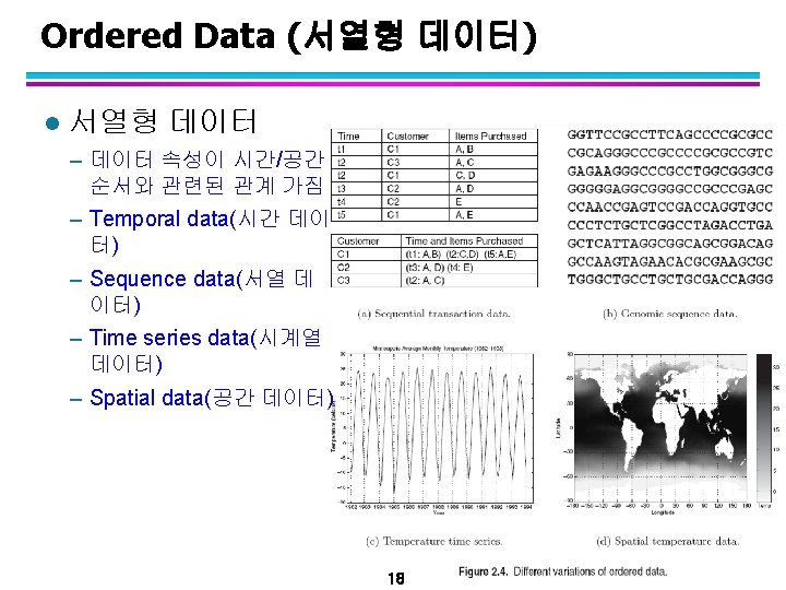
Types of data sets l l l Record – Data Matrix – Document Data – Transaction Data Graph – World Wide Web – Molecular Structures Ordered – Spatial Data – Temporal Data – Sequential Data – Genetic Sequence Data 10

Record Data l Data that consists of a collection of records, each of which consists of a fixed set of attributes 12

Data Matrix l If data objects have the same fixed set of numeric attributes, then the data objects can be thought of as points in a multi-dimensional space, where each dimension represents a distinct attribute l Such data set can be represented by an m by n matrix, where there are m rows, one for each object, and n columns, one for each attribute 13

Document Data l Each document becomes a `term' vector, – each term is a component (attribute) of the vector, – the value of each component is the number of times the corresponding term occurs in the document. 14

Transaction Data l A special type of record data, where – each record (transaction) involves a set of items. – For example, consider a grocery store. The set of products purchased by a customer during one shopping trip constitute a transaction, while the individual products that were purchased are the items. 15

Graph Data - Chemical Data l Examples: Benzene Molecule: C 6 H 6 17

2. 2 Data Quality (데이터 품질) What kinds of data quality problems? l How can we detect problems with the data? l What can we do about these problems? l l Examples of data quality problems: – Noise and outliers – missing values – duplicate data 19

Noise l Noise is the random component of a measurement error – It may involve the distortion of a value or the addition of spurious objects – Examples: distortion of a person’s voice when talking on a poor phone and “snow” on television screen Two Sine Waves 20 Two Sine Waves + random Noise

Outliers l Outliers are data objects with characteristics that are considerably different than most of the other data objects in the data set 21

Missing Values l l It is usual for an object to be missing one or more attribute values Reasons for missing values – Information is not collected (e. g. , people decline to give their age and weight) – Attributes may not be applicable to all cases (e. g. , annual income is not applicable to children) l Handling missing values – Estimate Missing Values (누락값 추정) – Eliminate Data Objects (누락값 제거) – Ignore the Missing Value During Analysis (분석 과정에서 누락값 무시) – Replace with all possible values (weighted by their probabilities) ( 누락값을 가능성있는 값으로 대체) 22

Duplicate Data (중복 데이터) l Data set may include data objects that are duplicates, or almost duplicates of one another – Major issue when merging data from heterogeous sources l Examples: – Same person with multiple email addresses l Data cleaning (데이터 정제) – Process of dealing with duplicate data issues 23

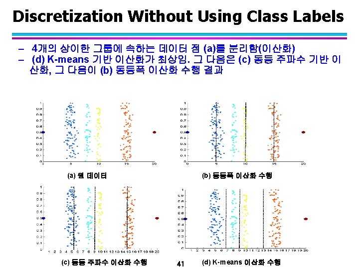
2. 3 Data Preprocessing(데이터 전처리) Aggregation(집합/집계/총계) l Sampling(표본 추출) l Dimensionality Reduction(차원 축소) l Feature subset selection(특징 부분집합 선택) l Feature creation(특징 생성) l Discretization and Binarization(이산화와 이진화) l Attribute Transformation(속성 변환) l 24

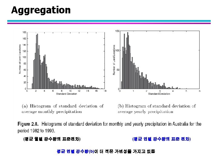
Aggregation l Combining two or more attributes (or objects) into a single attribute (or object) l Purpose – Data reduction u Reduce the number of attributes or objects – Change of scale u Cities aggregated into regions, states, countries, etc – More “stable” data u Aggregated data tends to have less variability 25

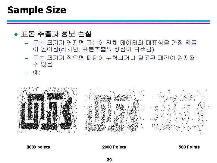
Sampling l Sampling is the main technique employed for data selection. – It is often used for both the preliminary investigation of the data and the final data analysis. l Statisticians sample because obtaining the entire set of data of interest is too expensive or time consuming. l Sampling is used in data mining because processing the entire set of data of interest is too expensive or time consuming. 27

Sampling … l The key principle for effective sampling is the following: – using a sample will work almost as well as using the entire data sets, if the sample is representative – A sample is representative if it has approximately the same property (of interest) as the original set of data 28

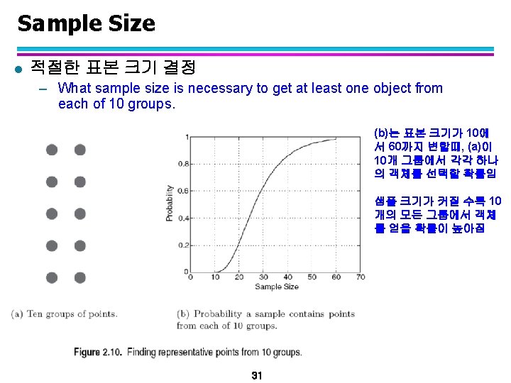
Types of Sampling l Simple Random Sampling(단순 임의 표본추출) – There is an equal probability of selecting any particular item l Sampling without replacement(무대체 표본추출) – As each item is selected, it is removed from the population l Sampling with replacement(대체 표본추출) – Objects are not removed from the population as they are selected for the sample. u In sampling with replacement, the same object can be picked up more than once l Stratified sampling(층화 표본추출) – Split the data into several partitions; then draw random samples from each partition (모집단을 층으로 나눈 후, 각 층에서 샘플링) – 층내에서는 동질적, 층간은 이질적 특성을 가지도록 하면 적은 비 용으로 더 정확한 추정 가능 29

Curse of Dimensionality l l l 차원이 증가하면 데이터는 그 차원이 차지하는 공간상 에서 점점더 sparse하게 됨 분석이 어려워짐 Classification에선 충분한 데이터 객체가 존재하지 않 아 모델 생성이 어려워짐 Clustering에선 clustering 의 핵심인 density와 두점 간의 distance 정보가 작아 서 군집화가 어려워짐 • Randomly generate 500 points • Compute difference between max and min distance between any pair of points 32

Dimensionality Reduction 기법 l Purpose: – Avoid curse of dimensionality – Reduce amount of time and memory required by data mining algorithms – Allow data to be more easily visualized – May help to eliminate irrelevant features or reduce noise l Techniques – Principle Component Analysis (주성분 분석) – Singular Value Decomposition(특이값 분해) – Others: supervised and non-linear techniques 33

Dimensionality Reduction: PCA l 최대한의 데이터 변이를 얻기 위함 – The Goal is to find a projection that captures the largest amount of variation in data x 2 e 34 x 1

Dimensionality Reduction: PCA l Find the eigenvectors of the covariance matrix – One of the most intuitive explanations of eigenvectors of a covariance matrix is that they are the directions in which the data varies the most. – Example) Each data sample is a 2 dimensional point with coordinates x, y. The eigenvectors of the covariance matrix of these data samples are the vectors u and v; – u : first eigenvector, v, the shorter arrow, is the second eigenvector • The first eigenvector is the direction in which the data varies the most, the second eigenvector is the direction of greatest variance among those that are orthogonal (perpendicular) to the first eigenvector. • The eigenvalues are the length of the arrows. 35

Feature Subset Selection(특징 부분집합 선택) l Another way to reduce dimensionality of data l Redundant features(중복 특징) – duplicate much or all of the information contained in one or more other attributes – Example: purchase price of a product and the amount of sales tax paid l Irrelevant features(비관련 특징) – contain no information that is useful for the data mining task at hand – Example: students' ID is often irrelevant to the task of predicting students' GPA 36

Feature Subset Selection l 특징 부분집합 선택 기법: – Brute-force approach: u Try all possible feature subsets as input to data mining algorithm – Embedded approaches: u Feature selection occurs naturally as part of the data mining algorithm – Filter approaches: u Features are selected before data mining algorithm is run – Wrapper approaches: u Use the data mining algorithm as a black box to find best subset of attributes 37

Feature Creation l Create new attributes that can capture the important information in a data set much more efficiently than the original attributes l Three general methodologies: – Feature Extraction(특징 추출) u domain-specific – Mapping Data to New Space(새로운 공간으로 데이터 매핑) – Feature Construction(특징 구축) u combining features 38

Mapping Data to a New Space – Fourier transform : sin/cos 함수로 time domain 신호 frequency domain으로 변환 – Wavelet transform : sin/cos함수뿐만 아니라, 다양한 wavelet 모 함수를 사용하여 변환함 Two Sine Waves + Noise 39 Frequency

Attribute Transformation l l It alters the data by replacing a selected attribute by one or more new attributes A function that maps the entire set of values of a given attribute to a new set of replacement values such that each old value can be identified with one of the new values – Simple functions: xk, log(x), ex, |x| – Standardization and Normalization, etc. 42

2. 4 Similarity and Dissimilarity(유사도와 비유사도) l Similarity – Numerical measure of how alike two data objects are. – Is higher when objects are more alike. – Often falls in the range [0, 1] l Dissimilarity – Numerical measure of how different are two data objects – Lower when objects are more alike – Minimum dissimilarity is often 0 – Upper limit varies l Proximity refers to a similarity or dissimilarity 43

Similarity/Dissimilarity for Simple Attributes p and q are the attribute values for two data objects.

Euclidean Distance l Euclidean Distance Where n is the number of dimensions (attributes) and pk and qk are, respectively, the kth attributes (components) or data objects p and q. l Standardization is necessary, if scales differ. 45

Euclidean Distance Matrix 46

Minkowski Distance l Minkowski Distance is a generalization of Euclidean Distance Where r is a parameter, n is the number of dimensions (attributes) and pk and qk are, respectively, the kth attributes (components) or data objects p and q. 47

Minkowski Distance: Examples l r = 1. City block : Manhattan norm, taxicab norm, L 1 norm – A common example of this is the Hamming distance, which is just the number of bits that are different between two binary vectors l r = 2. Euclidean distance L 2 norm l r . “supremum” (Lmax norm, L norm) distance. – This is the maximum difference between any component of the vectors l Do not confuse r with n, i. e. , all these distances are defined for all numbers of dimensions. 48

Minkowski Distance Matrix 49

Mahalanobis Distance § This is a measure of the distance between a point P and a distribution D § P가 분포 D의 평균으로부터 표준편차의 몇 배 떨어져 있는지를 알 수 있 음 For red points, the Euclidean distance is 14. 7, Mahalanobis distance is 6. 50

Mahalanobis Distance (example) If, in our single observation, X = 410 and Y = 400 (other data is not shown in this example), we would calculate the Mahalanobis distance for that single value as: < Calculation of Mahalanobis distance> < covariance matrix > Var(X)=std_dev(X)^2, Cov(X, Y)=E((X-u)(Y-v)) Cov(Y, X), Var(Y) 51

Mahalanobis Distance Covariance Matrix: C A: (0. 5, 0. 5) B B: (0, 1) A C: (1. 5, 1. 5) Mahal(A, B) = 5 Mahal(A, C) = 4

Common Properties of a Distance l Distances, such as the Euclidean distance, have some well known properties. 1. d(p, q) 0 for all p and q, and d(p, q) = 0 only if p = q. (Positive definiteness) 2. 3. d(p, q) = d(q, p) for all p and q. (Symmetry) d(p, r) d(p, q) + d(q, r) for all points p, q, and r. (Triangle Inequality) where d(p, q) is the distance (dissimilarity) between points (data objects), p and q. l A distance that satisfies these properties is a metric 53

Common Properties of a Similarity l Similarities, also have some well known properties. 1. s(p, q) = 1 (or maximum similarity) only if p = q. 2. s(p, q) = s(q, p) for all p and q. (Symmetry) where s(p, q) is the similarity between points (data objects), p and q. 54

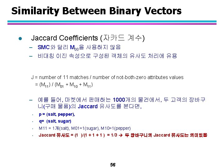
Similarity Between Binary Vectors l Common situation is that objects, p and q, have only binary attributes l Compute similarities using the following quantities M 01 = the number of attributes where p was 0 and q was 1 M 10 = the number of attributes where p was 1 and q was 0 M 00 = the number of attributes where p was 0 and q was 0 M 11 = the number of attributes where p was 1 and q was 1 Simple Matching Coefficients (단순 매칭 계수) l SMC = 매칭 속성의 수/속성의 수 = (M 11 + M 00) / (M 01 + M 10 + M 11 + M 00) - SMC는 p도 없고 q도 없는 속성까지 고려를 하고 있음 예를 들어, 마켓에서 판매하는 1000개의 물건에서, 두 고객(p, q)의 장바구니(구매 물품)의 SMC 유사도를 본다면, • p = (salt, pepper), • q= (salt, sugar) • M 11 = 1개(salt), M 00=(1000개 – 3), M 01=1(sugar), M 10=1(pepper) • SMC = (1 + 997)/(1 + 1 + 997) = 0. 998 의미없음 55

SMC versus Jaccard: Example p = 1 0 0 0 0 0 q = 0 0 0 1 M 01 = 2 (the number of attributes where p was 0 and q was 1) M 10 = 1 (the number of attributes where p was 1 and q was 0) M 00 = 7 (the number of attributes where p was 0 and q was 0) M 11 = 0 (the number of attributes where p was 1 and q was 1) SMC = (M 11 + M 00)/(M 01 + M 10 + M 11 + M 00) = (0+7) / (2+1+0+7) = 0. 7 J = (M 11) / (M 01 + M 10 + M 11) = 0 / (2 + 1 + 0) = 0 57

Cosine Similarity l If d 1 and d 2 are two document vectors, then cos( d 1, d 2 ) = (d 1 d 2) / ||d 1|| ||d 2|| , where indicates vector dot product and || is the length of vector d. l Example: d 1 = 3 2 0 5 0 0 0 2 0 0 d 2 = 1 0 0 0 1 0 2 d 1 d 2= 3*1 + 2*0 + 0*0 + 5*0 + 0*0 + 2*1 + 0*0 + 0*2 = 5 ||d 1|| = (3*3+2*2+0*0+5*5+0*0+0*0+2*2+0*0)0. 5 = (42) 0. 5 = 6. 481 ||d 2|| = (1*1+0*0+0*0+0*0+1*1+0*0+2*2) 0. 5 = (6) 0. 5 = 2. 245 cos( d 1, d 2 ) =. 3150 • Cosine 유사도가 0 이라는 것은 아무런 관련성 없음을 의미 58

Extended Jaccard Coefficient (Tanimoto) l Variation of Jaccard for continuous or count attributes – Reduces to Jaccard for binary attributes 59

Correlation measures the linear relationship between objects l To compute correlation, we standardize data objects, p and q, and then take their dot product l 60

Visually Evaluating Correlation -1에서 1의 상관도를 보여주 는 산포도(scatter plots) 61

General Approach for Combining Similarities l Sometimes attributes are of many different types, but an overall similarity is needed. 62

Using Weights to Combine Similarities l May not want to treat all attributes the same. – Use weights wk which are between 0 and 1 and sum to 1. 63

Density l Density-based clustering require a notion of density l Examples: – Euclidean density u Euclidean density = number of points per unit volume – Probability density – Graph-based density 64

Euclidean Density – Cell-based l Simplest approach is to divide region into a number of rectangular cells of equal volume and define density as # of points the cell contains 65

Euclidean Density – Center-based l Euclidean density is the number of points within a specified radius of the point 66