CSE 245 Computer Aided Circuit Simulation and Verification

CSE 245: Computer Aided Circuit Simulation and Verification Matrix Computations: Iterative Methods I Chung-Kuan Cheng

Outline o Introduction o Direct Methods o Iterative Methods n n n Formulations Projection Methods Krylov Space Methods Preconditioned Iterations Multigrid Methods Domain Decomposition Methods 2

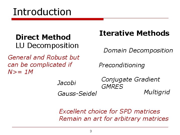
Introduction Iterative Methods Direct Method LU Decomposition Domain Decomposition General and Robust but can be complicated if N>= 1 M Preconditioning Conjugate Gradient Jacobi GMRES Multigrid Gauss-Seidel Excellent choice for SPD matrices Remain an art for arbitrary matrices 3

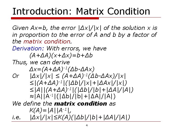
Introduction: Matrix Condition Given Ax=b, the error |∆x|/|x| of the solution x is in proportion to the error of A and b by a factor of the matrix condition. Derivation: With errors, we have (A+∆A)(x+∆x)=b+∆b Thus, we can derive ∆x=(A+∆A)-1(∆b-∆Ax) Or |∆x|/|x| ≤ (A+∆A)-1(∆b-∆Ax)/|x| ≤|(A+∆A)-1|(|∆b|/|x|+|∆Ax|/|x|) ≤|A||(A+∆A)-1|(|∆b|/|b|+|∆A|/|A|) ≈|A||A-1|(|∆b|/|b|+|∆A|/|A|) We define the matrix condition as K(A)=|A||A-1|, i. e. |∆x|/|x|≤K(A)(|∆b|/|b|+|∆A|/|A|) 4

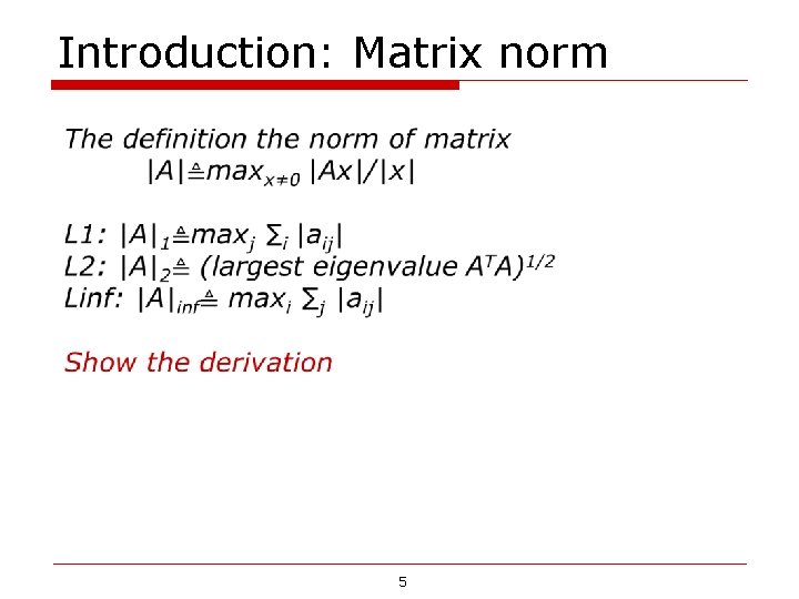
Introduction: Matrix norm 5

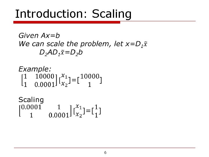
Introduction: Scaling 6

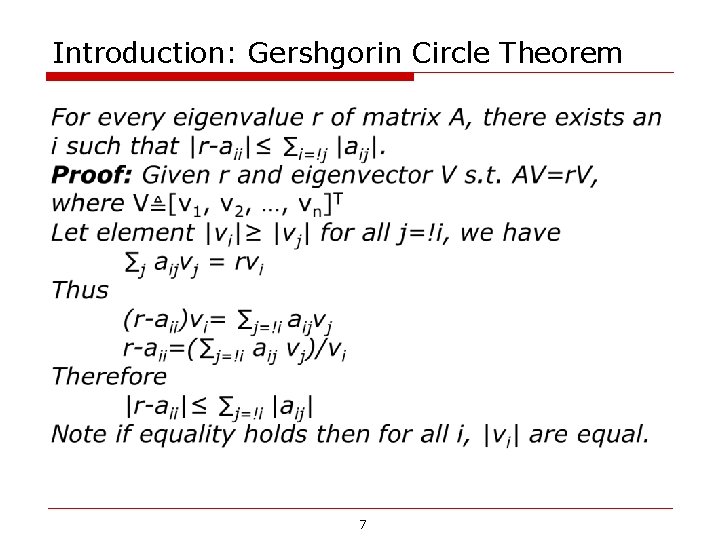
Introduction: Gershgorin Circle Theorem 7

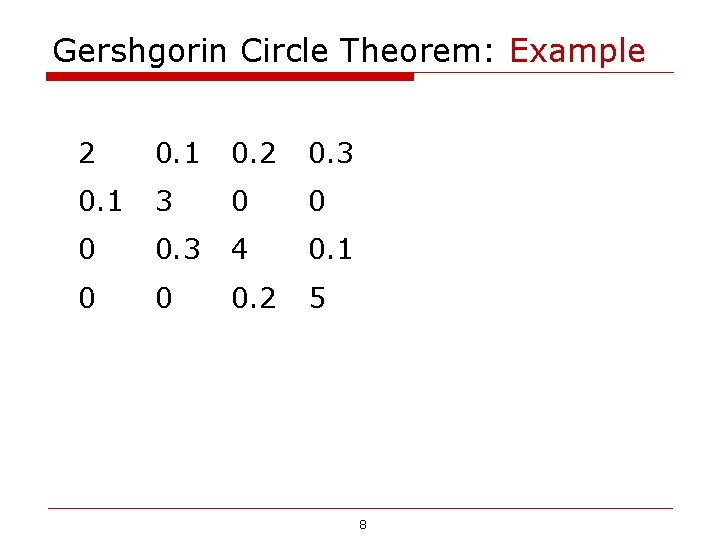
Gershgorin Circle Theorem: Example 2 0. 1 0. 2 0. 3 0. 1 3 0 0. 3 4 0. 1 0 0 0. 2 5 8

Iterative Methods Stationary: x(k+1) =Gx(k)+c where G and c do not depend on iteration count (k) Non Stationary: x(k+1) =x(k)+akp(k) where computation involves information that change at each iteration 9

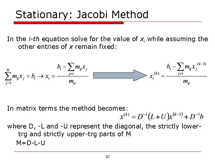
Stationary: Jacobi Method In the i-th equation solve for the value of xi while assuming the other entries of x remain fixed: In matrix terms the method becomes: where D, -L and -U represent the diagonal, the strictly lowertrg and strictly upper-trg parts of M M=D-L-U 10

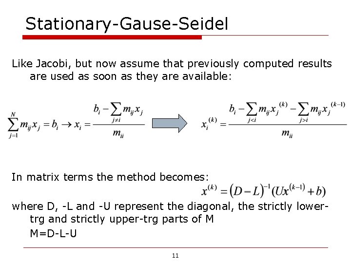
Stationary-Gause-Seidel Like Jacobi, but now assume that previously computed results are used as soon as they are available: In matrix terms the method becomes: where D, -L and -U represent the diagonal, the strictly lowertrg and strictly upper-trg parts of M M=D-L-U 11

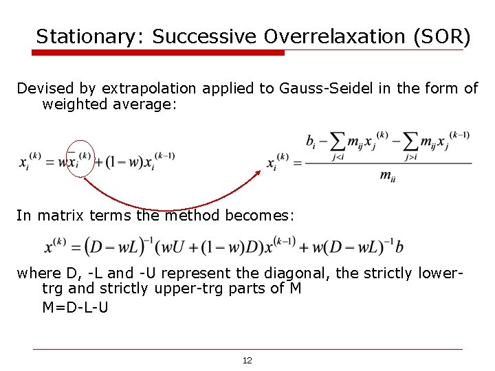
Stationary: Successive Overrelaxation (SOR) Devised by extrapolation applied to Gauss-Seidel in the form of weighted average: In matrix terms the method becomes: where D, -L and -U represent the diagonal, the strictly lowertrg and strictly upper-trg parts of M M=D-L-U 12

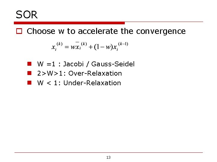
SOR o Choose w to accelerate the convergence n W =1 : Jacobi / Gauss-Seidel n 2>W>1: Over-Relaxation n W < 1: Under-Relaxation 13

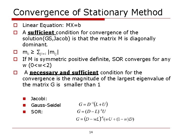
Convergence of Stationary Method o Linear Equation: MX=b o A sufficient condition for convergence of the solution(GS, Jacob) is that the matrix M is diagonally dominant. o mii ≥ ∑j!=i |mij| o If M is symmetric positive definite, SOR converges for any w (0<w<2) o A necessary and sufficient condition for the convergence is the magnitude of the largest eigenvalue of the matrix G is smaller than 1 n n n Jacobi: Gauss-Seidel SOR: 14

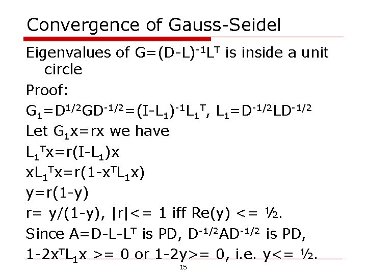
Convergence of Gauss-Seidel Eigenvalues of G=(D-L)-1 LT is inside a unit circle Proof: G 1=D 1/2 GD-1/2=(I-L 1)-1 L 1 T, L 1=D-1/2 LD-1/2 Let G 1 x=rx we have L 1 Tx=r(I-L 1)x x. L 1 Tx=r(1 -x. TL 1 x) y=r(1 -y) r= y/(1 -y), |r|<= 1 iff Re(y) <= ½. Since A=D-L-LT is PD, D-1/2 AD-1/2 is PD, 1 -2 x. TL 1 x >= 0 or 1 -2 y>= 0, i. e. y<= ½. 15

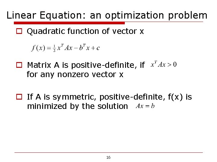
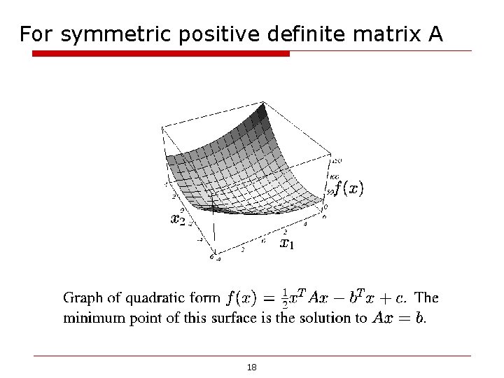
Linear Equation: an optimization problem o Quadratic function of vector x o Matrix A is positive-definite, if for any nonzero vector x o If A is symmetric, positive-definite, f(x) is minimized by the solution 16

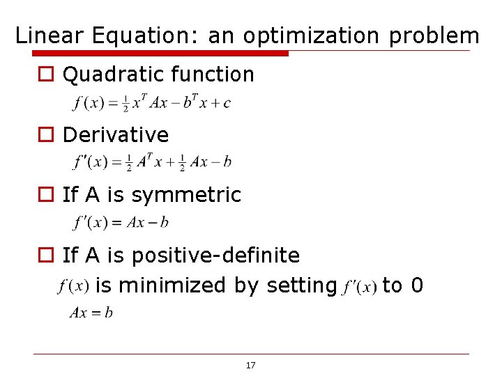
Linear Equation: an optimization problem o Quadratic function o Derivative o If A is symmetric o If A is positive-definite is minimized by setting 17 to 0

For symmetric positive definite matrix A 18

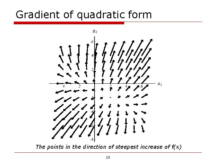
Gradient of quadratic form The points in the direction of steepest increase of f(x) 19

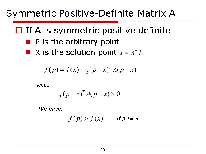
Symmetric Positive-Definite Matrix A o If A is symmetric positive definite n P is the arbitrary point n X is the solution point since We have, If p != x 20

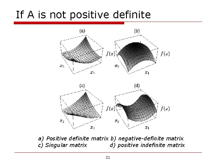
If A is not positive definite a) Positive definite matrix b) negative-definite matrix c) Singular matrix d) positive indefinite matrix 21

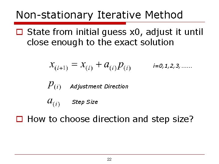
Non-stationary Iterative Method o State from initial guess x 0, adjust it until close enough to the exact solution i=0, 1, 2, 3, …… Adjustment Direction Step Size o How to choose direction and step size? 22

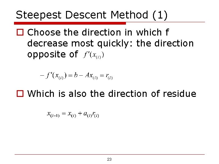
Steepest Descent Method (1) o Choose the direction in which f decrease most quickly: the direction opposite of o Which is also the direction of residue 23

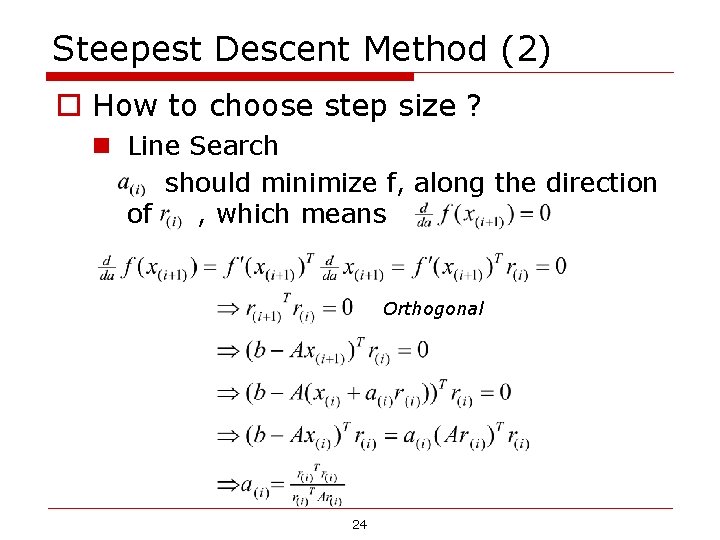
Steepest Descent Method (2) o How to choose step size ? n Line Search should minimize f, along the direction of , which means Orthogonal 24

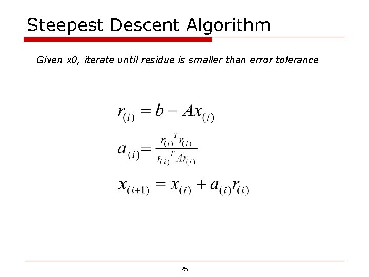
Steepest Descent Algorithm Given x 0, iterate until residue is smaller than error tolerance 25

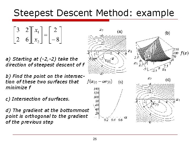
Steepest Descent Method: example a) Starting at (-2, -2) take the direction of steepest descent of f b) Find the point on the intersection of these two surfaces that minimize f c) Intersection of surfaces. d) The gradient at the bottommost point is orthogonal to the gradient of the previous step 26

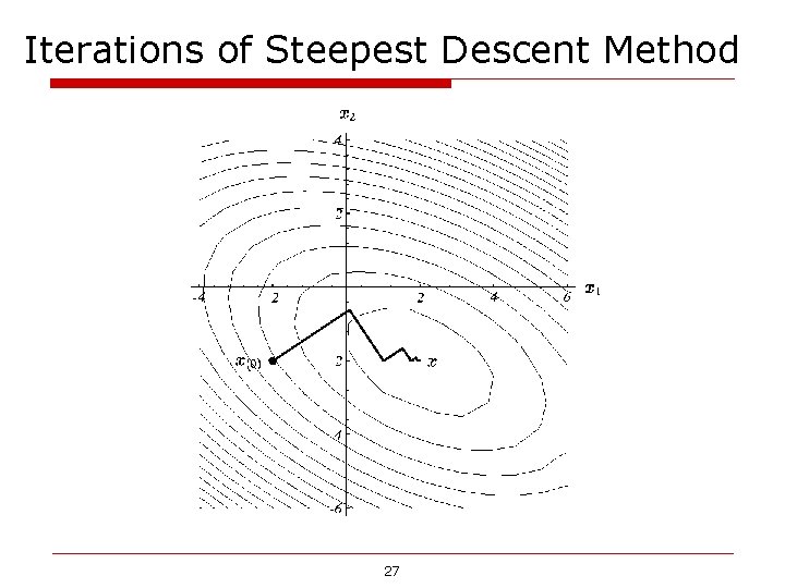
Iterations of Steepest Descent Method 27

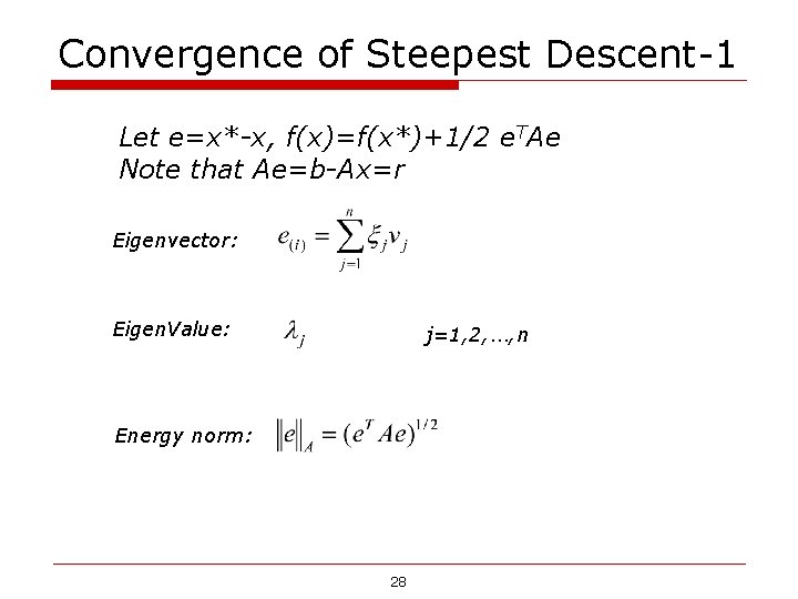
Convergence of Steepest Descent-1 Let e=x*-x, f(x)=f(x*)+1/2 e. TAe Note that Ae=b-Ax=r Eigenvector: Eigen. Value: j=1, 2, …, n Energy norm: 28

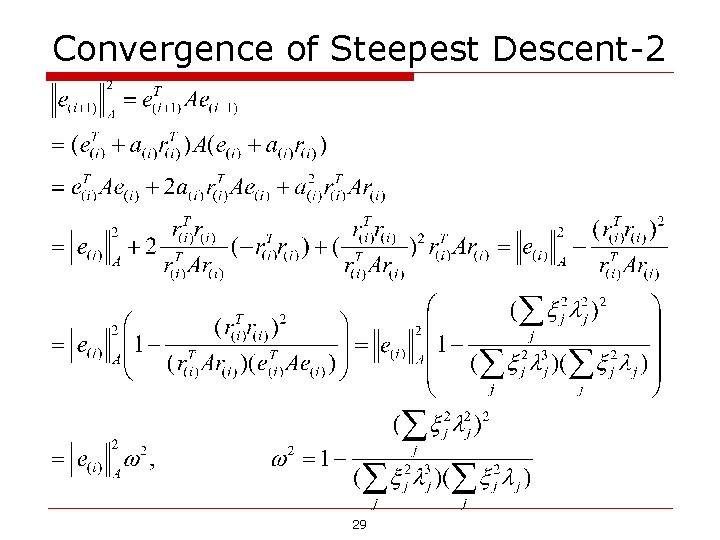
Convergence of Steepest Descent-2 29

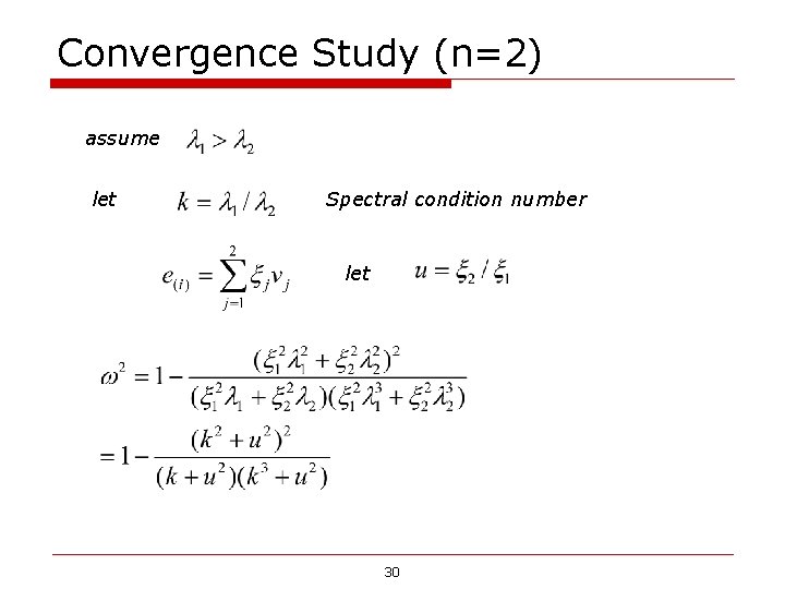
Convergence Study (n=2) assume let Spectral condition number let 30

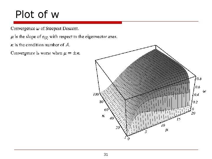
Plot of w 31

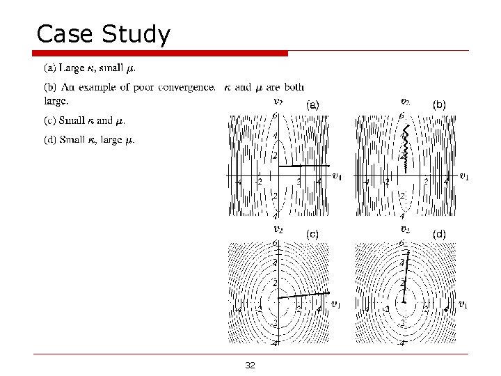
Case Study 32

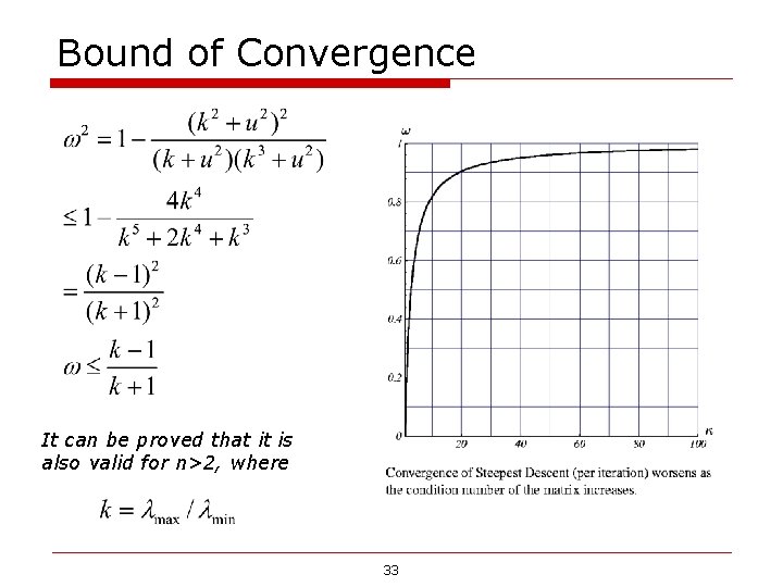
Bound of Convergence It can be proved that it is also valid for n>2, where 33