CSE 202 Algorithms Fall 2002 Instructor Larry Carter

CSE 202 - Algorithms • Fall 2002 • • • Instructor: Larry Carter carter@cs. ucsd. edu Office hours (4101 AP&M) Tu & Th 3: 30 – 5: 00 (or whenever) • TA: John-Paul Fryckman 9/26/2002 CSE 202 - Intro • jfryckm@cs. ucsd. edu

What we’ll study General Techniques Divide and Conquer, Dynamic Programming, Hashing, Greedy Algorithms, Reduction to other problems, . . . Specific Problems Sorting, shortest paths, max flow, sorting, . . . Various Paradigms Probabilistic algorithms Alternate models of computation NP Completeness 2 CSE 202 - Intro

Sounds like my undergrad course. . . • Going over same material twice is good! • We’ll probably go deeper – mathematical formalisms – modified assumptions – assorted topics every computer scientist should know. 3 CSE 202 - Intro

Logistics • Textbook: Introduction to Algorithms, 2 nd edition – Cormen, Leiserson, Rivest & Stein – First edition probably OK (new chapter K ~ old chapter (K+1). ) • Written work – Individual homeworks – Group homeworks – In-class Midterm – Final (oral? take-home? ) • Grades – A: Demonstrate mastery of material. – B (or B+ or B-): Typical grade. Understand most of material, solve most routine problems and some hard ones. – C: Really don’t “get it”. 4 – D, F: Gave up. CSE 202 - Intro

Logistics • Classes will include “lecture” (with overheads), “discussion” (at board), and “exercises” (at your seat). – I’d prefer you pay attention, think, ask questions, and participate in discussions rather than taking notes. • Website: //www. cs. ucsd. edu/classes/fa 02/cse 202 -b –. pdf and. ps of “lectures”. (Sometimes available before class. ) – Homeworks, announcements, etc. too – You are responsible for checking website • Be sure to register for the class email list – I’ll use it to send out urgent messages, like HW corrections – Directions on class webpage 5 CSE 202 - Intro

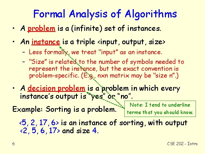
Formal Analysis of Algorithms • A problem is a (infinite) set of instances. • An instance is a triple <input, output, size> – Less formally, we treat “input” as an instance. – “Size” is related to the number of symbols needed to represent the instance, but the exact convention is problem-specific. (E. g. , nxn matrix may be “size n”. ) • A decision problem is a problem in which every instance’s output is “yes” or “no”. Example: Sorting is a problem. Note: I tend to underline terms that you should know. <5, 2, 17, 6> is an instance of sorting, with output <2, 5, 6, 17> and size 4. 6 CSE 202 - Intro

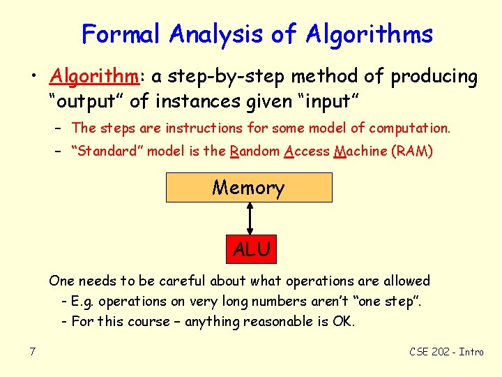
Formal Analysis of Algorithms • Algorithm: a step-by-step method of producing “output” of instances given “input” – The steps are instructions for some model of computation. – “Standard” model is the Random Access Machine (RAM) Memory ALU One needs to be careful about what operations are allowed - E. g. operations on very long numbers aren’t “one step”. - For this course – anything reasonable is OK. 7 CSE 202 - Intro

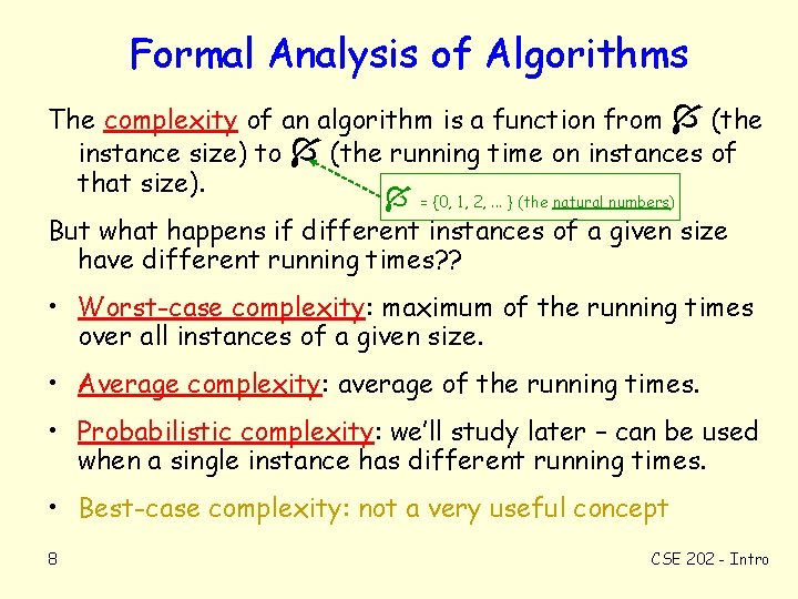
Formal Analysis of Algorithms The complexity of an algorithm is a function from (the instance size) to (the running time on instances of that size). = {0, 1, 2, . . . } (the natural numbers) But what happens if different instances of a given size have different running times? ? • Worst-case complexity: maximum of the running times over all instances of a given size. • Average complexity: average of the running times. • Probabilistic complexity: we’ll study later – can be used when a single instance has different running times. • Best-case complexity: not a very useful concept 8 CSE 202 - Intro

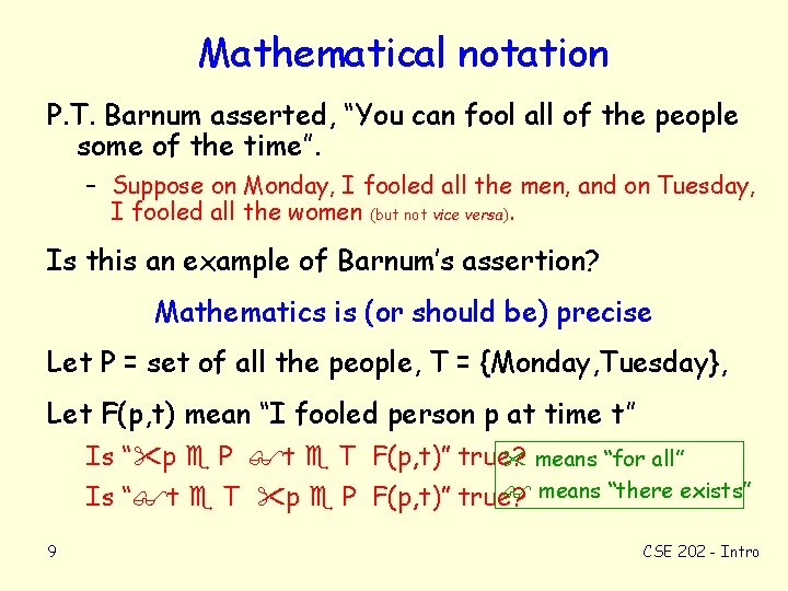
Mathematical notation P. T. Barnum asserted, “You can fool all of the people some of the time”. – Suppose on Monday, I fooled all the men, and on Tuesday, I fooled all the women (but not vice versa). Is this an example of Barnum’s assertion? Mathematics is (or should be) precise Let P = set of all the people, T = {Monday, Tuesday}, Let F(p, t) mean “I fooled person p at time t” Is “ p P t T F(p, t)” true? means “for all” means “there exists” Is “ t T p P F(p, t)” true? 9 CSE 202 - Intro

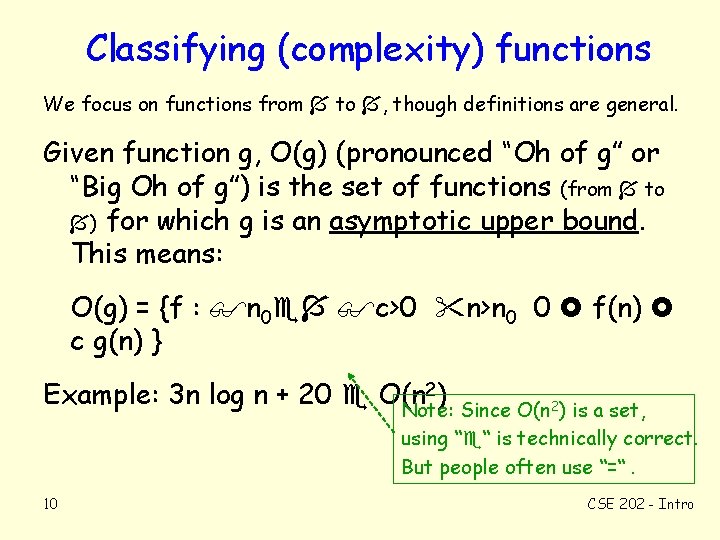
Classifying (complexity) functions We focus on functions from to , though definitions are general. Given function g, O(g) (pronounced “Oh of g” or “Big Oh of g”) is the set of functions (from to ) for which g is an asymptotic upper bound. This means: O(g) = {f : n 0 c>0 n>n 0 0 f(n) c g(n) } 2) Example: 3 n log n + 20 O(n Note: Since O(n 2) is a set, using “ “ is technically correct. But people often use “=“. 10 CSE 202 - Intro

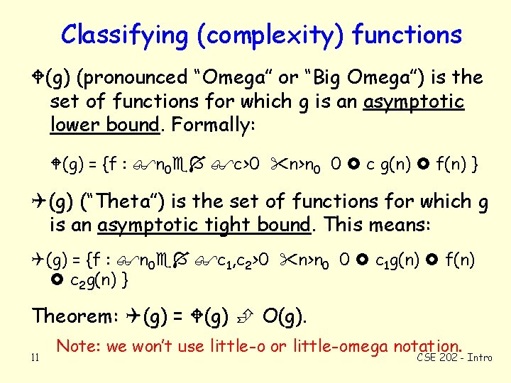
Classifying (complexity) functions (g) (pronounced “Omega” or “Big Omega”) is the set of functions for which g is an asymptotic lower bound. Formally: (g) = {f : n 0 c>0 n>n 0 0 c g(n) f(n) } (g) (“Theta”) is the set of functions for which g is an asymptotic tight bound. This means: (g) = {f : n 0 c 1, c 2>0 n>n 0 0 c 1 g(n) f(n) c 2 g(n) } Theorem: (g) = (g) O(g). 11 Note: we won’t use little-o or little-omega notation. CSE 202 - Intro

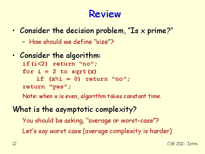
Review • Consider the decision problem, “Is x prime? ” – How should we define “size”? • Consider the algorithm: if(i<2) return “no”; for i = 2 to sqrt(x) if (x%i = 0) return “no”; return “yes”; Note: when x is even, algorithm takes constant time. What is the asymptotic complexity? You should be asking, “average or worst-case”? Let’s say worst case (average complexity is harder) 12 CSE 202 - Intro

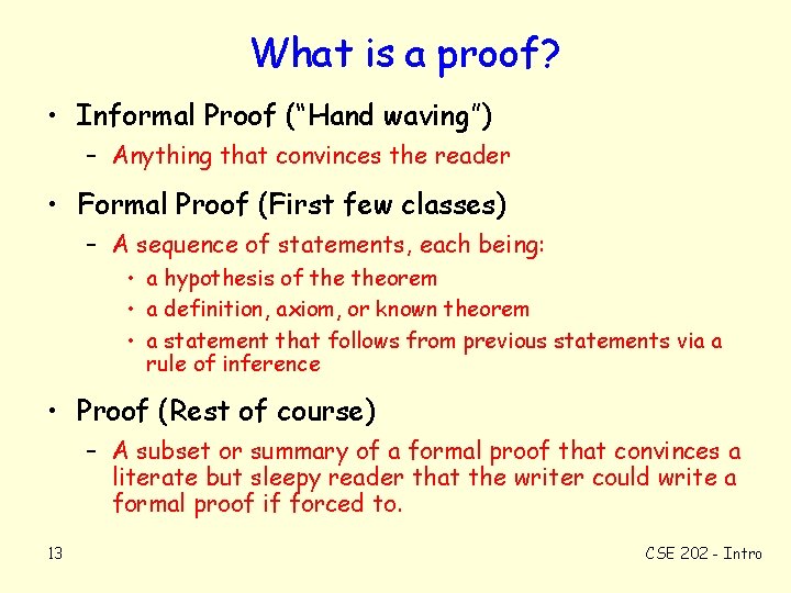
What is a proof? • Informal Proof (“Hand waving”) – Anything that convinces the reader • Formal Proof (First few classes) – A sequence of statements, each being: • a hypothesis of theorem • a definition, axiom, or known theorem • a statement that follows from previous statements via a rule of inference • Proof (Rest of course) – A subset or summary of a formal proof that convinces a literate but sleepy reader that the writer could write a formal proof if forced to. 13 CSE 202 - Intro

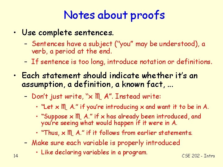
Notes about proofs • Use complete sentences. – Sentences have a subject (“you” may be understood), a verb, a period at the end. – If sentence is too long, introduce notation or definitions. • Each statement should indicate whether it’s an assumption, a definition, a known fact, . . . – Don’t just write, “x A”. Instead write: • “Let x A. ” if you’re introducing x and want it to be in A. • “Suppose x A. ” if x has already been introduced, and you’re seeing what would happen if it were in A. • “Thus, x A. ” if it follows from earlier statements. – Make sure each variable is properly introduced 14 • Like declaring variables in a program. CSE 202 - Intro

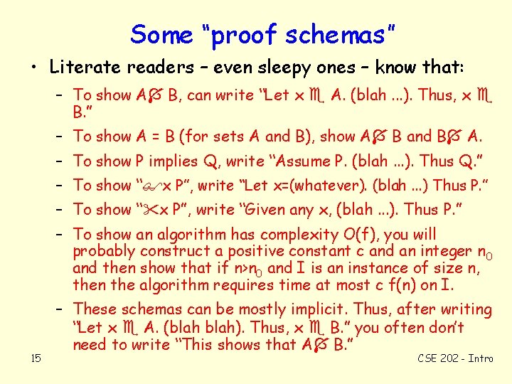
Some “proof schemas” • Literate readers – even sleepy ones – know that: – To show A B, can write “Let x A. (blah. . . ). Thus, x B. ” – To show A = B (for sets A and B), show A B and B A. – To show P implies Q, write “Assume P. (blah. . . ). Thus Q. ” – To show “ x P”, write “Let x=(whatever). (blah. . . ) Thus P. ” – To show “ x P”, write “Given any x, (blah. . . ). Thus P. ” – To show an algorithm has complexity O(f), you will probably construct a positive constant c and an integer n 0 and then show that if n>n 0 and I is an instance of size n, then the algorithm requires time at most c f(n) on I. 15 – These schemas can be mostly implicit. Thus, after writing “Let x A. (blah). Thus, x B. ” you often don’t need to write “This shows that A B. ” CSE 202 - Intro

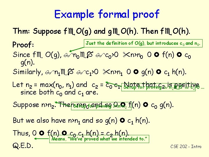
Example formal proof Thm: Suppose f O(g) and g O(h). Then f O(h). Proof: Just the definition of O(g), but introduces c 0 and n 0. Since f O(g), n 0 c 0>0 n>n 0 0 f(n) c 0 g(n). Similarly, n 1 c 1>0 n>n 1 0 g(n) c 1 h(n). Let n 2 = max(n 0, n 1) and c 2 = c 0 c 1. Setup Noteforthat c 2 n is 2 positive proving c 2>0. . . since both c 0 and c 1 are. Suppose n>n 2. Then. Setup n>n 0 forand so n>n 0 2. . . f(n) c 0 g(n). proving But we also have n>n 1 and so g(n) c 1 h(n). Thus, 0 f(n) c 0 c 1 h(n) = c 2 h(n). Q. E. D. 16 Means, “We’ve proved what we intended to. ” CSE 202 - Intro

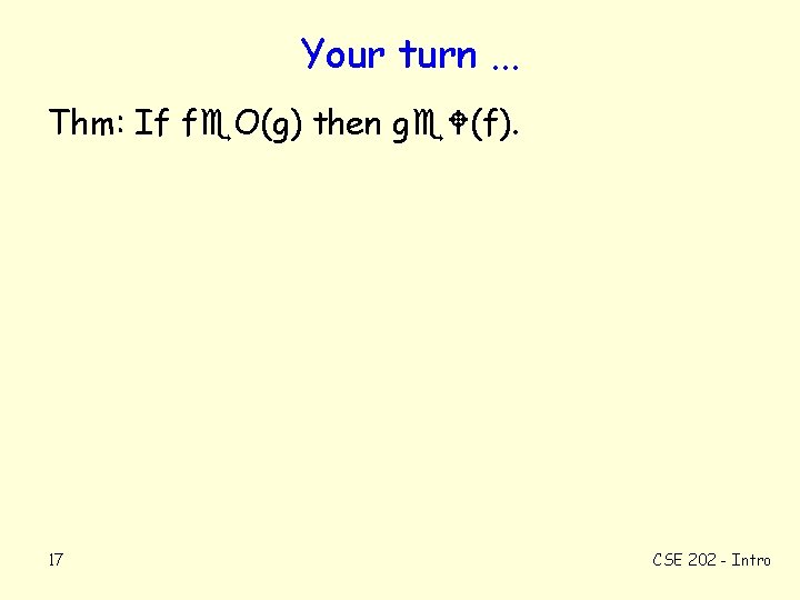
Your turn. . . Thm: If f O(g) then g (f). 17 CSE 202 - Intro

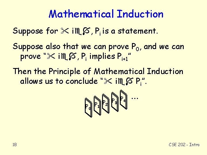
Mathematical Induction Suppose for i , Pi is a statement. Suppose also that we can prove P 0, and we can prove “ i , Pi implies Pi+1” Then the Principle of Mathematical Induction allows us to conclude “ i Pi”. P 0 18 P 1 P 2 P 3 P 4 . . . CSE 202 - Intro

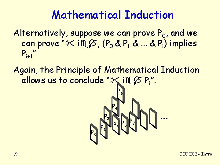
Mathematical Induction Alternatively, suppose we can prove P 0, and we can prove “ i , (P 0 & P 1 &. . . & Pi) implies Pi+1” Again, the Principle of Mathematical Induction allows us to conclude “ i Pi”. P 6 P 4 P 2 P 0 19 P 1 P P 3 P 5 7 . . . CSE 202 - Intro

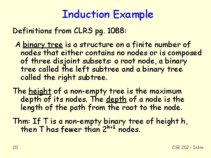
Induction Example Definitions from CLRS pg. 1088: A binary tree is a structure on a finite number of nodes that either contains no nodes or is composed of three disjoint subsets: a root node, a binary tree called the left subtree and a binary tree called the right subtree. The height of a non-empty tree is the maximum depth of its nodes. The depth of a node is the length of the path from the root to the node. Thm: If T is a non-empty binary tree of height h, then T has fewer than 2 h+1 nodes. 20 CSE 202 - Intro

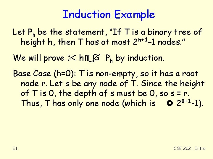
Induction Example Let Ph be the statement, “If T is a binary tree of height h, then T has at most 2 h+1– 1 nodes. ” We will prove h Ph by induction. Base Case (h=0): T is non-empty, so it has a root node r. Let s be any node of T. Since the height of T is 0, the depth of s must be 0, so s = r. Thus, T has only one node (which is 20+1 -1). 21 CSE 202 - Intro

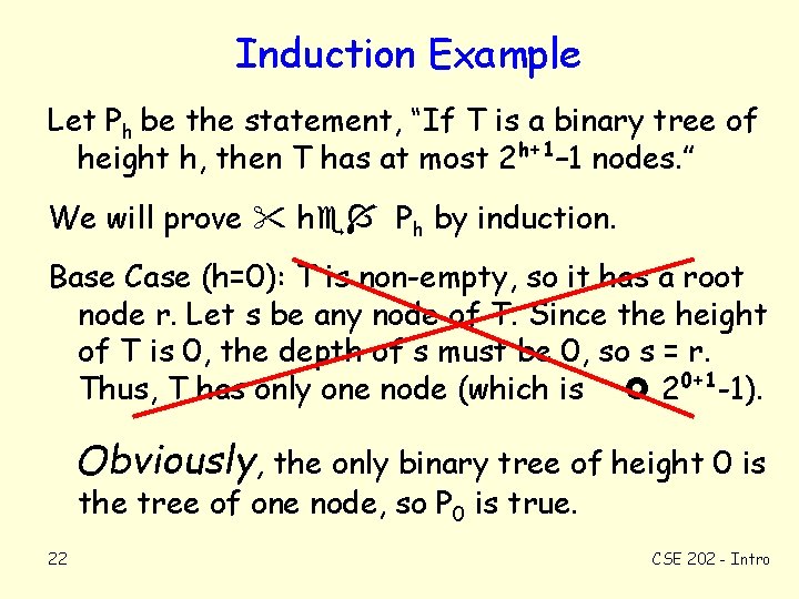
Induction Example Let Ph be the statement, “If T is a binary tree of height h, then T has at most 2 h+1– 1 nodes. ” We will prove h Ph by induction. Base Case (h=0): T is non-empty, so it has a root node r. Let s be any node of T. Since the height of T is 0, the depth of s must be 0, so s = r. Thus, T has only one node (which is 20+1 -1). Obviously, the only binary tree of height 0 is the tree of one node, so P 0 is true. 22 CSE 202 - Intro

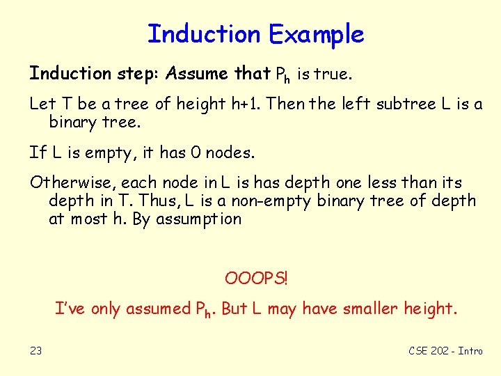
Induction Example Induction step: Assume that Ph is true. Let T be a tree of height h+1. Then the left subtree L is a binary tree. If L is empty, it has 0 nodes. Otherwise, each node in L is has depth one less than its depth in T. Thus, L is a non-empty binary tree of depth at most h. By assumption OOOPS! I’ve only assumed Ph. But L may have smaller height. 23 CSE 202 - Intro

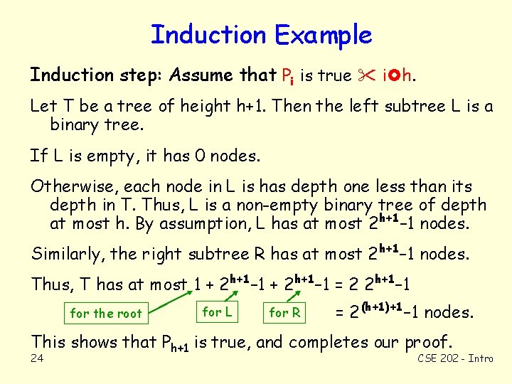
Induction Example Induction step: Assume that Pi is true i h. Let T be a tree of height h+1. Then the left subtree L is a binary tree. If L is empty, it has 0 nodes. Otherwise, each node in L is has depth one less than its depth in T. Thus, L is a non-empty binary tree of depth at most h. By assumption, L has at most 2 h+1– 1 nodes. Similarly, the right subtree R has at most 2 h+1– 1 nodes. Thus, T has at most 1 + 2 h+1– 1 = 2 2 h+1– 1 for the root for L for R = 2 (h+1)+1– 1 nodes. This shows that Ph+1 is true, and completes our proof. 24 CSE 202 - Intro