CS 654 Digital Image Analysis Lecture 5 Pixels

CS 654: Digital Image Analysis Lecture 5: Pixels Relationships

Recap of Lecture 4 • Different pixel relationships • Neighbourhood • Connectivity • Adjacency • Path • Connected component labelling

Outline • Different distance measures • Application of distance measures • Arithmetic and logical operations on images

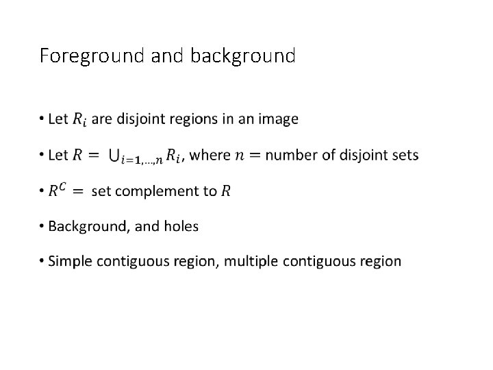
Region and boundary • A region is a set of pixels in which there is a path between any pair of pixels • Points within a region are contiguous: reflexive, symmetric and transitive • Decomposition of set • Connected component labeling

Foreground and background •

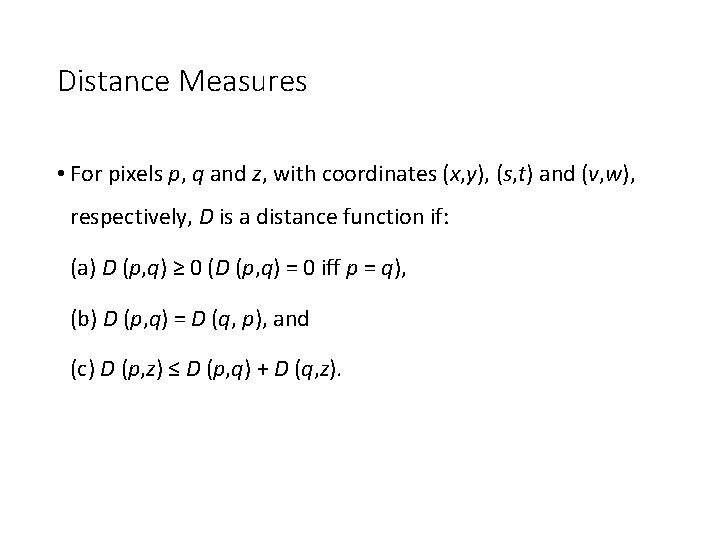
Distance Measures • For pixels p, q and z, with coordinates (x, y), (s, t) and (v, w), respectively, D is a distance function if: (a) D (p, q) ≥ 0 (D (p, q) = 0 iff p = q), (b) D (p, q) = D (q, p), and (c) D (p, z) ≤ D (p, q) + D (q, z).

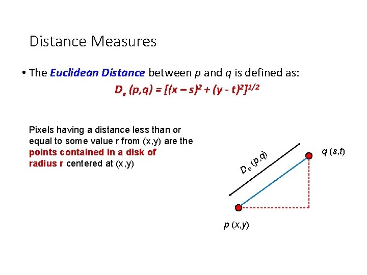
Distance Measures • The Euclidean Distance between p and q is defined as: De (p, q) = [(x – s)2 + (y - t)2]1/2 Pixels having a distance less than or equal to some value r from (x, y) are the points contained in a disk of radius r centered at (x, y) De p (x, y) (p ) , q q (s, t)

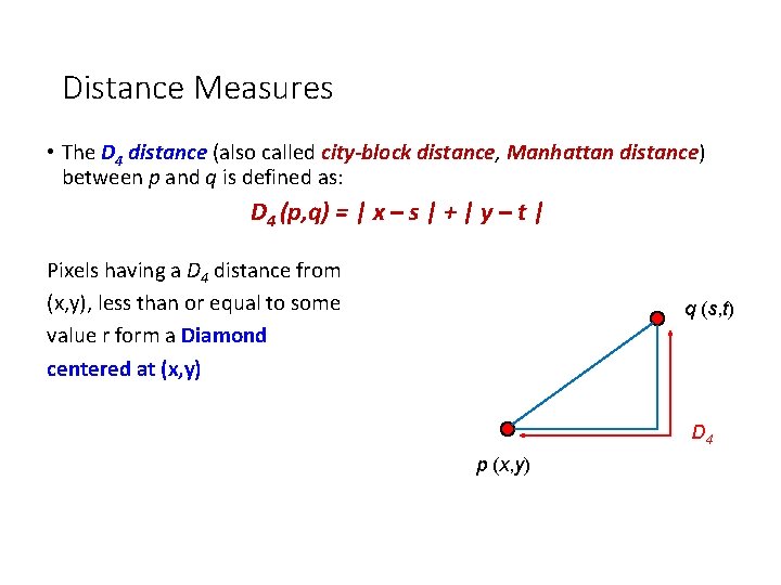
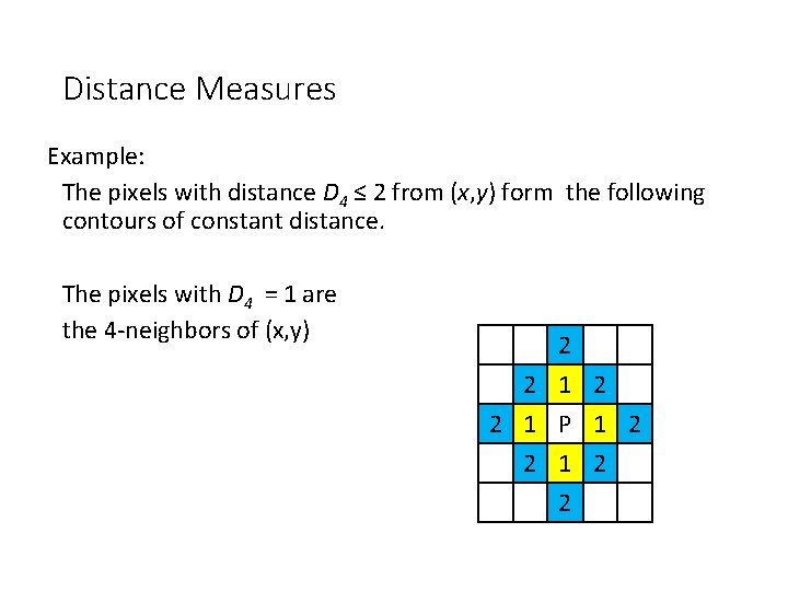
Distance Measures • The D 4 distance (also called city-block distance, Manhattan distance) between p and q is defined as: D 4 (p, q) = | x – s | + | y – t | Pixels having a D 4 distance from (x, y), less than or equal to some value r form a Diamond centered at (x, y) q (s, t) D 4 p (x, y)

Distance Measures Example: The pixels with distance D 4 ≤ 2 from (x, y) form the following contours of constant distance. The pixels with D 4 = 1 are the 4 -neighbors of (x, y) 2 2 1 P 1 2 2

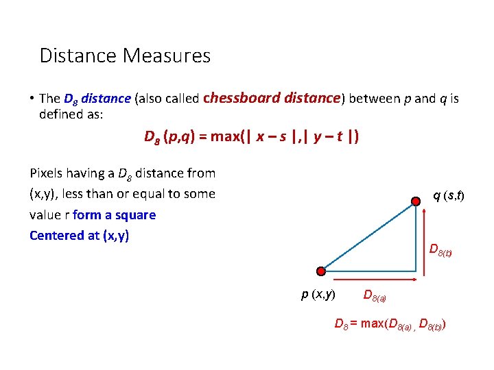
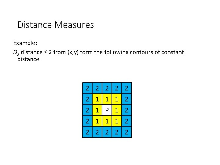
Distance Measures • The D 8 distance (also called chessboard distance) between p and q is defined as: D 8 (p, q) = max(| x – s |, | y – t |) Pixels having a D 8 distance from (x, y), less than or equal to some value r form a square Centered at (x, y) q (s, t) D 8(b) p (x, y) D 8(a) D 8 = max(D 8(a) , D 8(b))

Distance Measures Example: D 8 distance ≤ 2 from (x, y) form the following contours of constant distance. 2 2 2 1 1 1 2 1 P 1 2 1 1 1 2 2 2 2 2

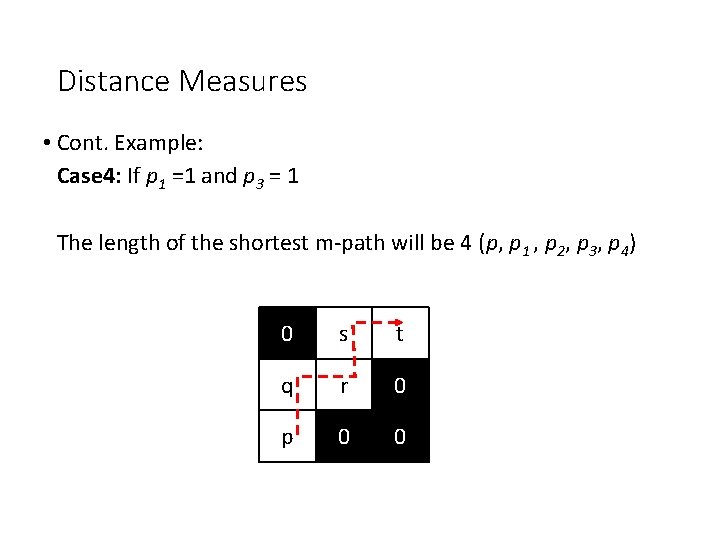
Distance Measures • Dm distance: is defined as the shortest m-path between the points. In this case, the distance between two pixels will depend on the values of the pixels along the path, as well as the values of their neighbors.

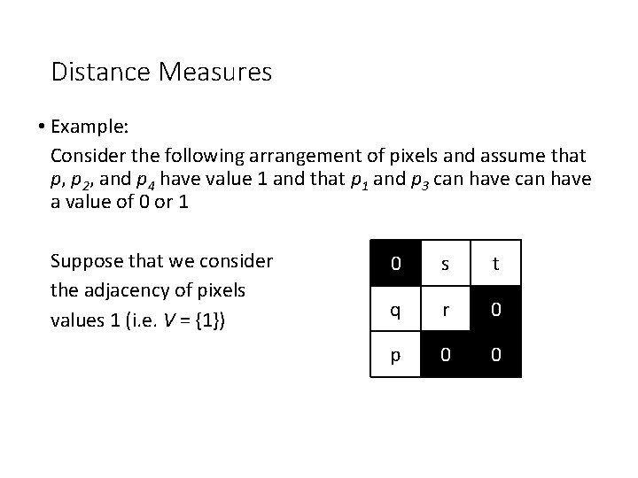
Distance Measures • Example: Consider the following arrangement of pixels and assume that p, p 2, and p 4 have value 1 and that p 1 and p 3 can have a value of 0 or 1 Suppose that we consider the adjacency of pixels values 1 (i. e. V = {1}) 0 s t q r 0 p 0 0

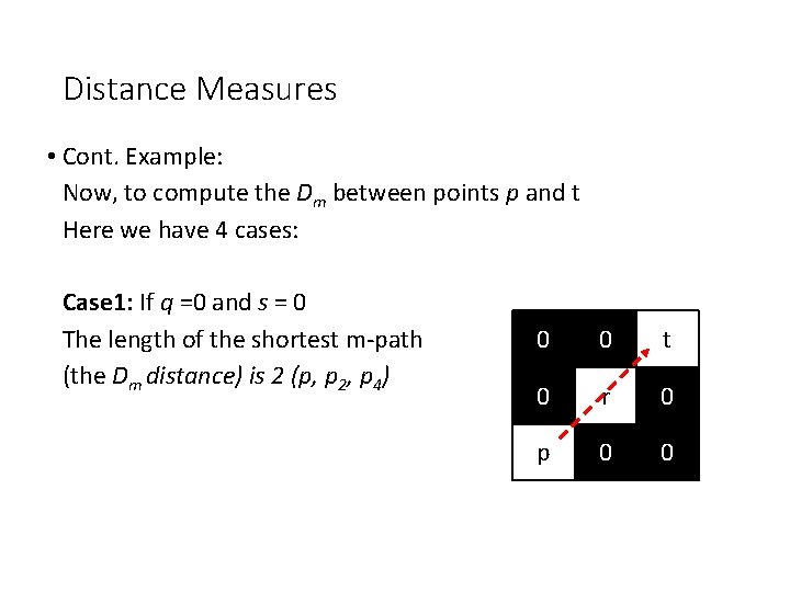
Distance Measures • Cont. Example: Now, to compute the Dm between points p and t Here we have 4 cases: Case 1: If q =0 and s = 0 The length of the shortest m-path (the Dm distance) is 2 (p, p 2, p 4) 0 0 t 0 r 0 p 0 0

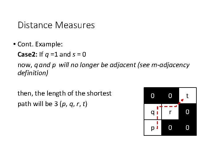
Distance Measures • Cont. Example: Case 2: If q =1 and s = 0 now, q and p will no longer be adjacent (see m-adjacency definition) then, the length of the shortest path will be 3 (p, q, r, t) 0 0 t q r 0 p 0 0

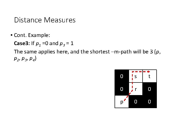
Distance Measures • Cont. Example: Case 3: If p 1 =0 and p 3 = 1 The same applies here, and the shortest –m-path will be 3 (p, p 2, p 3, p 4) 0 s t 0 r 0 p 0 0

Distance Measures • Cont. Example: Case 4: If p 1 =1 and p 3 = 1 The length of the shortest m-path will be 4 (p, p 1 , p 2, p 3, p 4) 0 s t q r 0 p 0 0

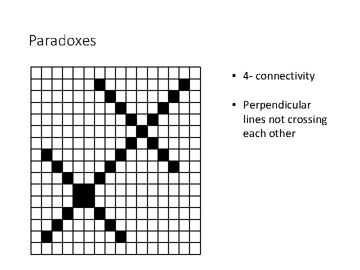
Paradoxes • 4 - connectivity • Perpendicular lines not crossing each other

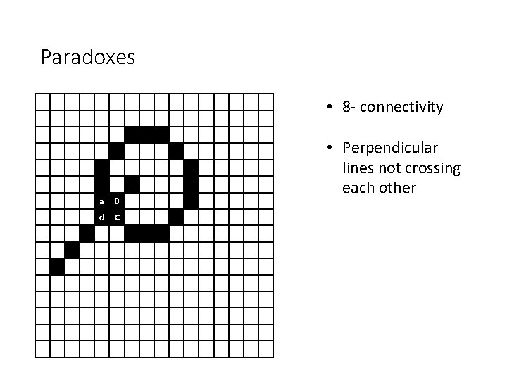
Paradoxes • 8 - connectivity a B d C • Perpendicular lines not crossing each other

Application of distance measure: Shape matching • Distance transform is an operator normally only applied to binary images. • The result of the transform is a gray-level image that looks similar to the input image • Except that the grey level intensities of points inside foreground regions are changed to show the distance to the closest boundary from each point.

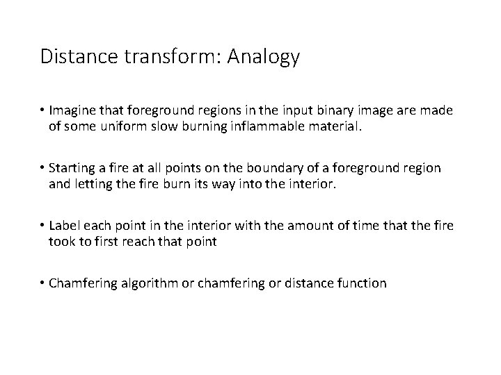
Distance transform: Analogy • Imagine that foreground regions in the input binary image are made of some uniform slow burning inflammable material. • Starting a fire at all points on the boundary of a foreground region and letting the fire burn its way into the interior. • Label each point in the interior with the amount of time that the fire took to first reach that point • Chamfering algorithm or chamfering or distance function

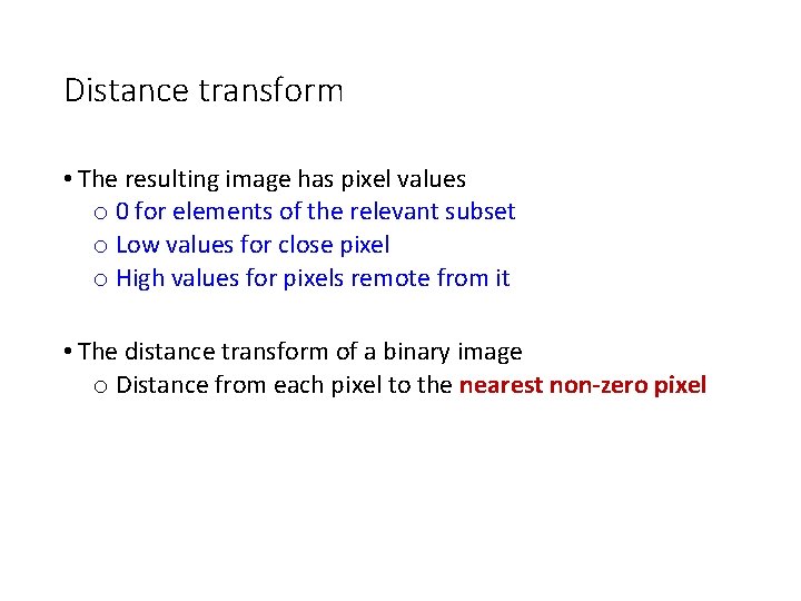
Distance transform • The resulting image has pixel values o 0 for elements of the relevant subset o Low values for close pixel o High values for pixels remote from it • The distance transform of a binary image o Distance from each pixel to the nearest non-zero pixel

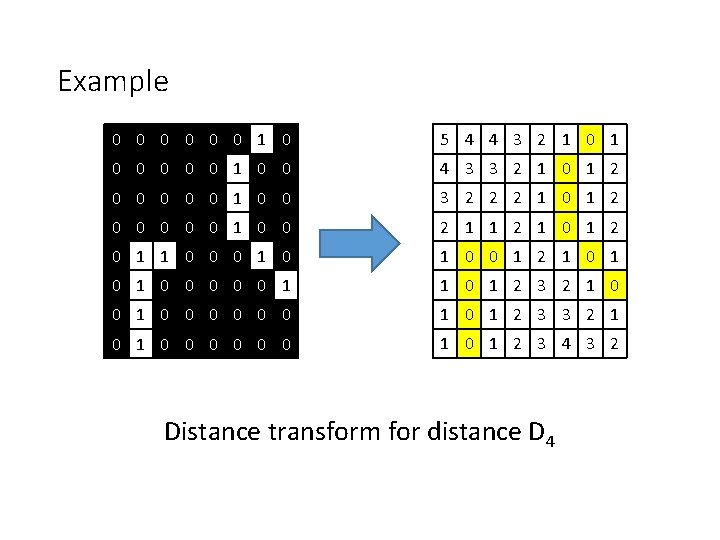
Example 0 0 0 1 0 5 4 4 3 2 1 0 0 0 1 0 0 4 3 3 2 1 0 1 2 0 0 0 1 0 0 3 2 2 2 1 0 1 2 0 0 0 1 0 0 2 1 1 2 1 0 1 2 0 1 1 0 0 0 1 2 1 0 1 0 0 0 1 1 0 1 2 3 2 1 0 0 0 0 1 0 1 2 3 3 2 1 0 0 0 0 1 2 3 4 3 2 Distance transform for distance D 4

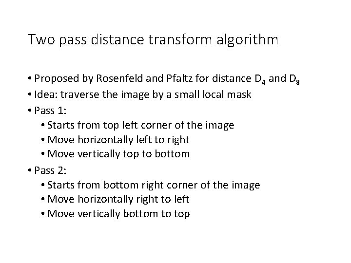
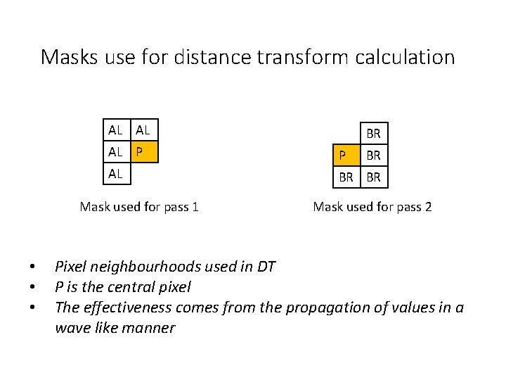
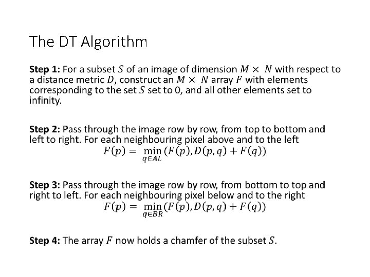
Two pass distance transform algorithm • Proposed by Rosenfeld and Pfaltz for distance D 4 and D 8 • Idea: traverse the image by a small local mask • Pass 1: • Starts from top left corner of the image • Move horizontally left to right • Move vertically top to bottom • Pass 2: • Starts from bottom right corner of the image • Move horizontally right to left • Move vertically bottom to top

Masks use for distance transform calculation AL AL AL P P AL BR BR Mask used for pass 1 • • • BR BR Mask used for pass 2 Pixel neighbourhoods used in DT P is the central pixel The effectiveness comes from the propagation of values in a wave like manner

The DT Algorithm •

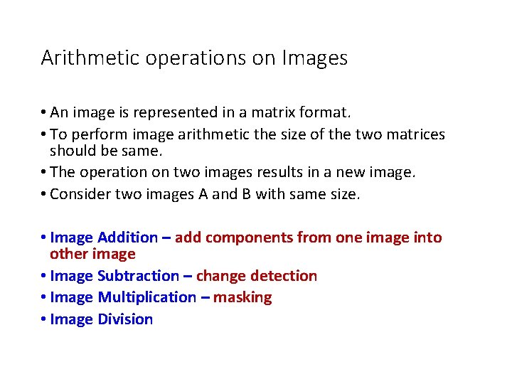
Arithmetic operations on Images • An image is represented in a matrix format. • To perform image arithmetic the size of the two matrices should be same. • The operation on two images results in a new image. • Consider two images A and B with same size. • Image Addition – add components from one image into other image • Image Subtraction – change detection • Image Multiplication – masking • Image Division

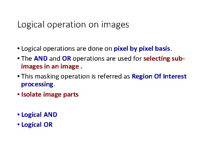
Logical operation on images • Logical operations are done on pixel by pixel basis. • The AND and OR operations are used for selecting subimages in an image. • This masking operation is referred as Region Of Interest processing. • Isolate image parts • Logical AND • Logical OR

Thank you Next Lecture: Basic transformations