CS 326 A Motion Planning NonHolonomic Motion Planning

CS 326 A: Motion Planning Non-Holonomic Motion Planning

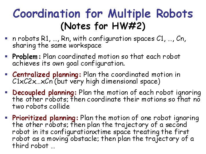
Coordination for Multiple Robots (Notes for HW#2) § n robots R 1, …, Rn, with configuration spaces C 1, …, Cn, sharing the same workspace § Problem: Plan coordinated motion so that each robot achieves its own goal configuration. § Centralized planning: Plan the coordinated motion in C 1 x. C 2 x…x. Cn (but very high dimensional space) § Decoupled planning: Plan the motion of each robot ignoring the other robots; then coordinate their motions so that no two robots collide § Prioritized planning: Plan the motion of one robot ignoring the other robots; then plan the trajectory of a second robot in its configurationxtime space treating the first robot as a moving obstacle; then plan the trajectory of a third robot …

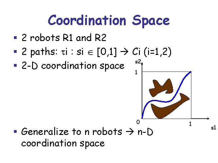
Coordination Space § 2 robots R 1 and R 2 § 2 paths: ti : si [0, 1] Ci (i=1, 2) s 2 § 2 -D coordination space 1 0 § Generalize to n robots n-D coordination space 1 s 1

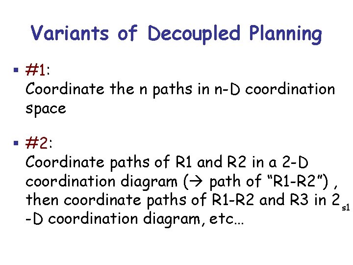
Variants of Decoupled Planning § #1: Coordinate the n paths in n-D coordination space § #2: Coordinate paths of R 1 and R 2 in a 2 -D coordination diagram ( path of “R 1 -R 2”) , then coordinate paths of R 1 -R 2 and R 3 in 2 s 1 -D coordination diagram, etc…

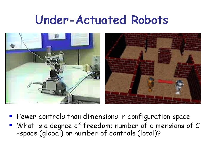
Under-Actuated Robots § Fewer controls than dimensions in configuration space § What is a degree of freedom: number of dimensions of C -space (global) or number of controls (local)?

How can m controls make it possible to span a C-space with n > m dimensions? By exploiting mechanics properties: - Rolling-with-no-sliding contact (friction), e. g. : car, bicycle, roller skate - Conservation of angular momentum: satellite robot, under-actuated robot, cat - Others: submarine, plane, object pushing Why is it useful? - Fewer actuators (less weight) - Design simplicity - Convenience (think about driving a car with 3 controls!)

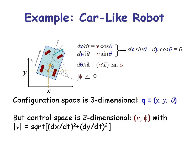
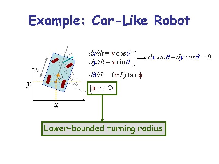
Example: Car-Like Robot dx/dt = v cosq dy/dt = v sinq f y q dq/dt = (v/L) tan f q f L dx sinq – dy cosq = 0 |f| < F x Configuration space is 3 -dimensional: q = (x, y, q) But control space is 2 -dimensional: (v, f) with |v| = sqrt[(dx/dt)2+(dy/dt)2]

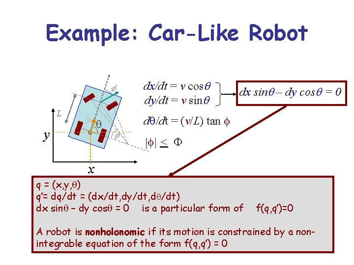
Example: Car-Like Robot dx/dt = v cosq dy/dt = v sinq f L q y dx sinq – dy cosq = 0 dq/dt = (v/L) tan f q |f| < F f x q = (x, y, q) q’= dq/dt = (dx/dt, dy/dt, dq/dt) dx sinq – dy cosq = 0 is a particular form of f(q, q’)=0 A robot is nonholonomic if its motion is constrained by a nonintegrable equation of the form f(q, q’) = 0

Example: Car-Like Robot dx/dt = v cosq dy/dt = v sinq f L q y dx sinq – dy cosq = 0 dq/dt = (v/L) tan f q |f| < F f x Lower-bounded turning radius

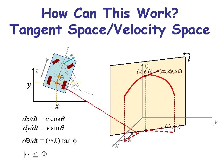
How Can This Work? Tangent Space/Velocity Space f L q y q (x, y, q) q (dx, dy, dq) f x dx/dt = v cosq dy/dt = v sinq dq/dt = (v/L) tan f |f| < F (dx, dy) x q y

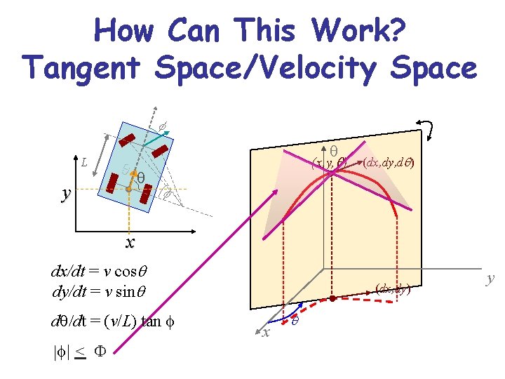
How Can This Work? Tangent Space/Velocity Space f L q y q (x, y, q) q (dx, dy, dq) f x dx/dt = v cosq dy/dt = v sinq dq/dt = (v/L) tan f |f| < F (dx, dy) x q y

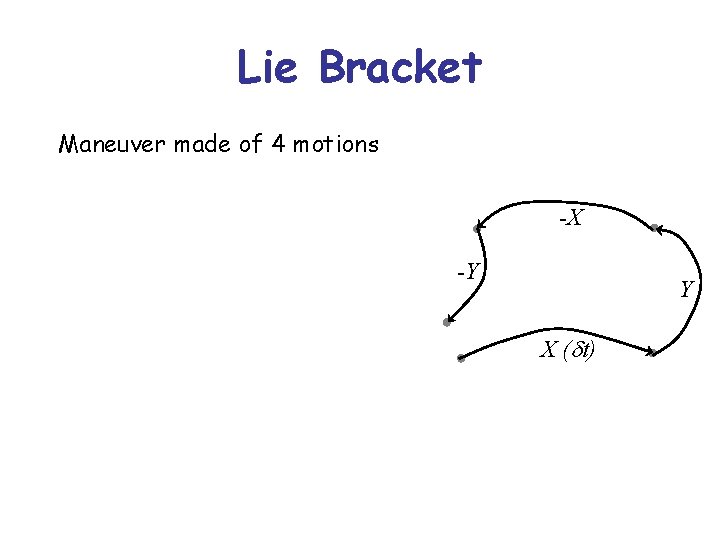
Lie Bracket Maneuver made of 4 motions -X -Y Y X (dt)

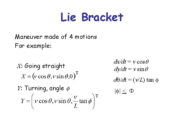
Lie Bracket Maneuver made of 4 motions For example: dx/dt = v cosq dy/dt = v sinq X: Going straight T dq/dt = (v/L) tan f Y: Turning, angle f T |f| < F

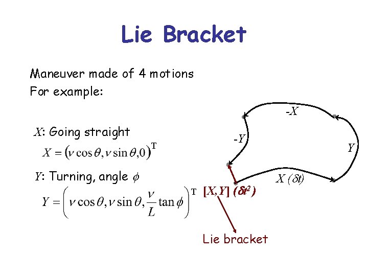
Lie Bracket Maneuver made of 4 motions For example: -X X: Going straight -Y T Y: Turning, angle f T [X, Y] (dt 2 ) Lie bracket Y X (dt)

Lie Bracket [X, Y] = d. Y. X – d. X. Y X 1/ x X 1/ y X 1/ q d. X = X 2/ x X 2/ y X 1/ q X 2/ x X 2/ y X 2/ q [X, Y] Lin(X, Y) the motion constraint is nonholonomic -X -Y [X, Y] (dt 2 ) Lie bracket Y X (dt)

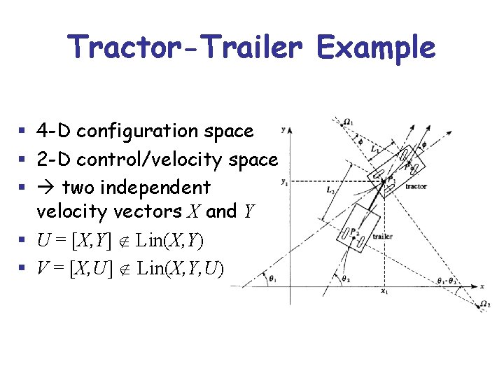
Tractor-Trailer Example § 4 -D configuration space § 2 -D control/velocity space § two independent velocity vectors X and Y § U = [X, Y] Lin(X, Y) § V = [X, U] Lin(X, Y, U)

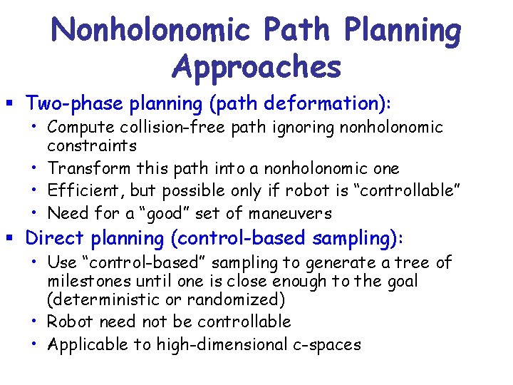
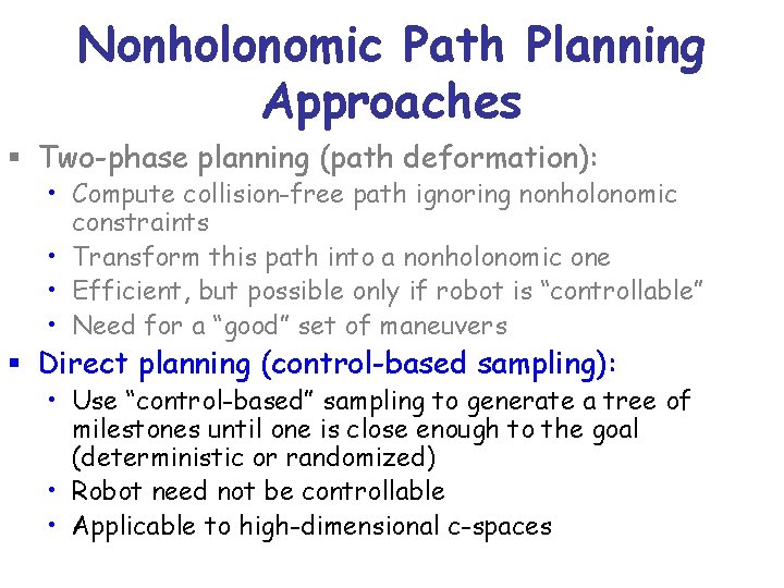
Nonholonomic Path Planning Approaches § Two-phase planning (path deformation): • Compute collision-free path ignoring nonholonomic constraints • Transform this path into a nonholonomic one • Efficient, but possible only if robot is “controllable” • Need for a “good” set of maneuvers § Direct planning (control-based sampling): • Use “control-based” sampling to generate a tree of milestones until one is close enough to the goal (deterministic or randomized) • Robot need not be controllable • Applicable to high-dimensional c-spaces

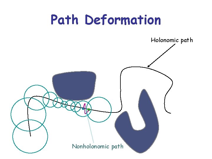
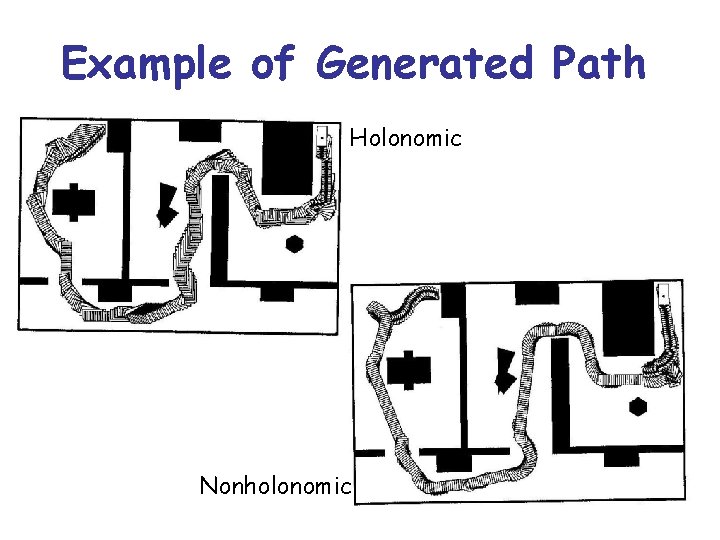
Path Deformation Holonomic path Nonholonomic path

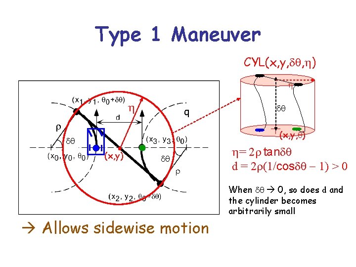
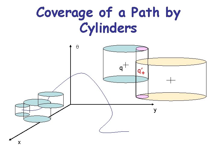
Type 1 Maneuver CYL(x, y, dq, h) h h q r dq (x, y, q) dq (x, y) dq r Allows sidewise motion h= 2 r tandq d = 2 r(1/cosdq - 1) > 0 When dq 0, so does d and the cylinder becomes arbitrarily small

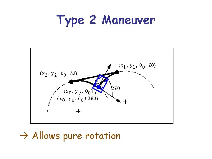
Type 2 Maneuver Allows pure rotation

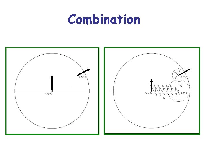
Combination

Coverage of a Path by Cylinders q q q’+ y x

Path Examples

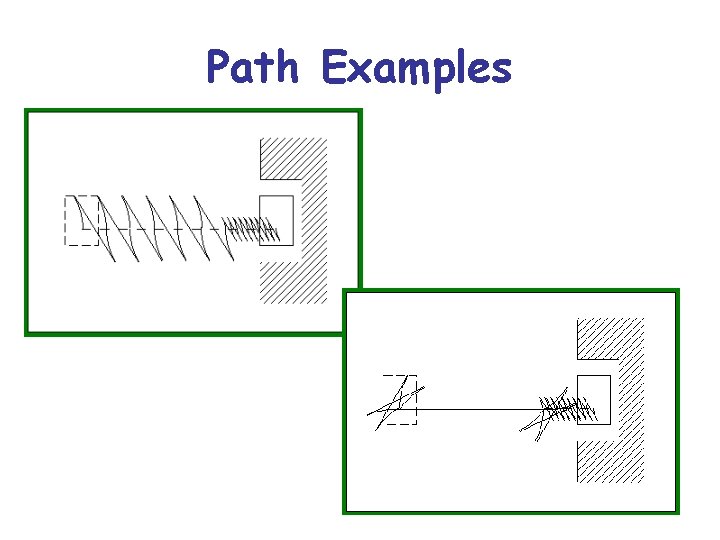
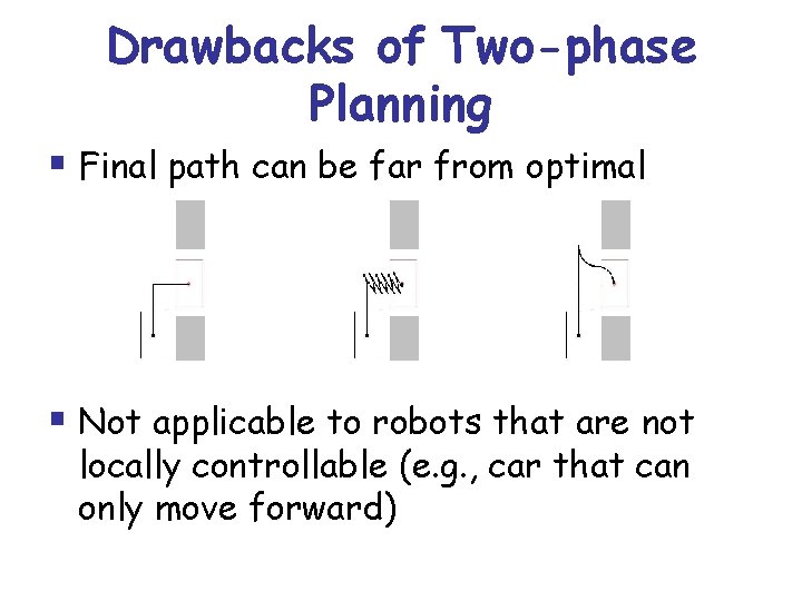
Drawbacks of Two-phase Planning § Final path can be far from optimal § Not applicable to robots that are not locally controllable (e. g. , car that can only move forward)

Reeds and Shepp Paths

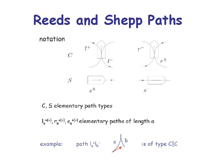
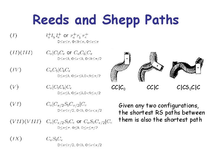
Reeds and Shepp Paths CC|C 0 CC|C C|CS 0 C|C Given any two configurations, the shortest RS paths between them is also the shortest path

Example of Generated Path Holonomic Nonholonomic

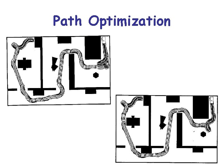
Path Optimization

Nonholonomic Path Planning Approaches § Two-phase planning (path deformation): • Compute collision-free path ignoring nonholonomic constraints • Transform this path into a nonholonomic one • Efficient, but possible only if robot is “controllable” • Need for a “good” set of maneuvers § Direct planning (control-based sampling): • Use “control-based” sampling to generate a tree of milestones until one is close enough to the goal (deterministic or randomized) • Robot need not be controllable • Applicable to high-dimensional c-spaces

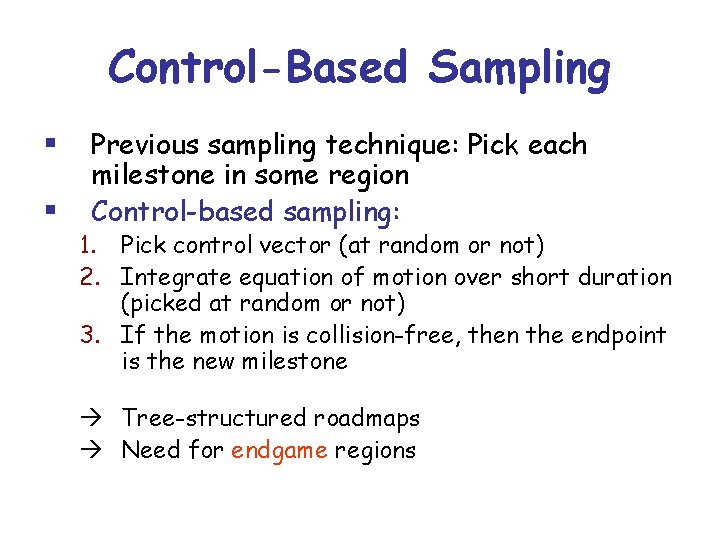
Control-Based Sampling § § Previous sampling technique: Pick each milestone in some region Control-based sampling: 1. Pick control vector (at random or not) 2. Integrate equation of motion over short duration (picked at random or not) 3. If the motion is collision-free, then the endpoint is the new milestone Tree-structured roadmaps Need for endgame regions

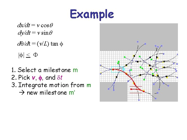
dx/dt = v cosq dy/dt = v sinq Example dq/dt = (v/L) tan f |f| < F 1. Select a milestone m 2. Pick v, f, and dt 3. Integrate motion from m new milestone m’

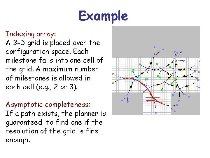
Example Indexing array: A 3 -D grid is placed over the configuration space. Each milestone falls into one cell of the grid. A maximum number of milestones is allowed in each cell (e. g. , 2 or 3). Asymptotic completeness: If a path exists, the planner is guaranteed to find one if the resolution of the grid is fine enough.

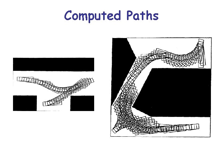
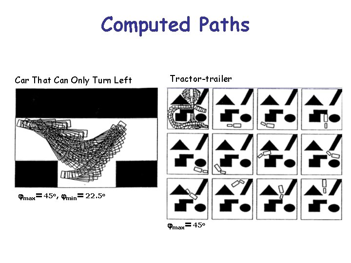
Computed Paths

Computed Paths Car That Can Only Turn Left Tractor-trailer jmax=45 o, jmin=22. 5 o jmax=45 o

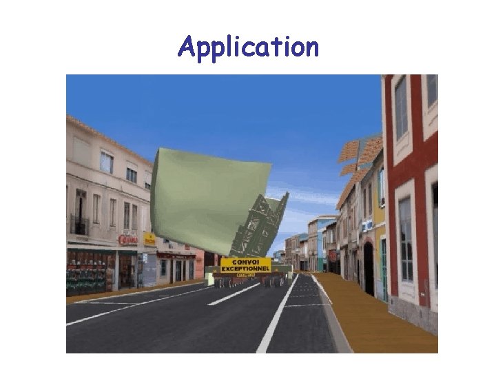
Application

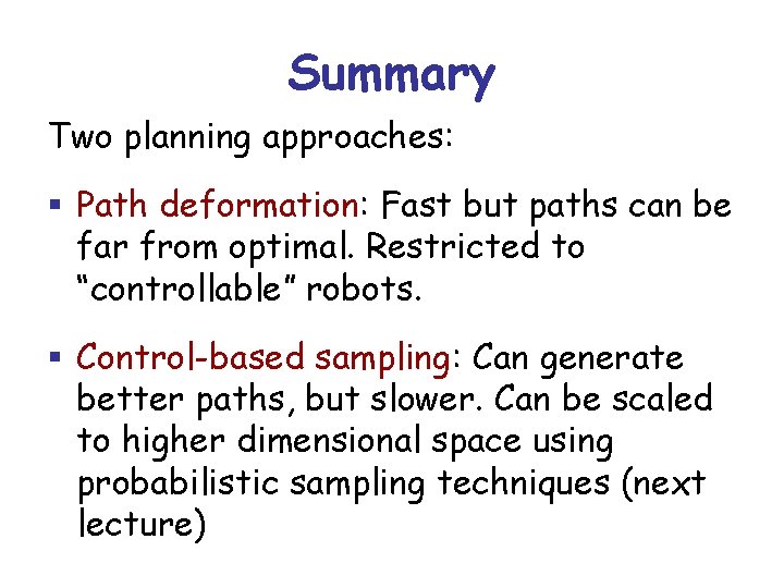
Summary Two planning approaches: § Path deformation: Fast but paths can be far from optimal. Restricted to “controllable” robots. § Control-based sampling: Can generate better paths, but slower. Can be scaled to higher dimensional space using probabilistic sampling techniques (next lecture)