Computer Architecture Lec 2 Introduction Review from last

Computer Architecture Lec 2 - Introduction

Review from last lecture • Computer Architecture >> instruction sets • Computer Architecture skill sets are different – 5 Quantitative principles of design – Quantitative approach to design – Solid interfaces that really work – Technology tracking and anticipation • 446 to learn new skills, transition to research • Computer Science at the crossroads from sequential to parallel computing – Salvation requires innovation in many fields, including computer architecture 10/23/2021 2

Review: Computer Architecture brings • Other fields often borrow ideas from architecture • Quantitative Principles of Design 1. Take Advantage of Parallelism 2. Principle of Locality 3. Focus on the Common Case 4. Amdahl’s Law 5. The Processor Performance Equation • Careful, quantitative comparisons – Define, quantity, and summarize relative performance – Define and quantity relative cost – Define and quantity dependability – Define and quantity power • Culture of anticipating and exploiting advances in technology • Culture of well-defined interfaces that are carefully implemented and thoroughly checked 10/23/2021 3

Outline • Review • Technology Trends: Culture of tracking, anticipating and exploiting advances in technology • Careful, quantitative comparisons: 1. Define, quantity, and summarize relative performance 2. Define and quantity relative cost 3. Define and quantity dependability 4. Define and quantity power 10/23/2021 CS 252 -s 06, Lec 02 -intro 4

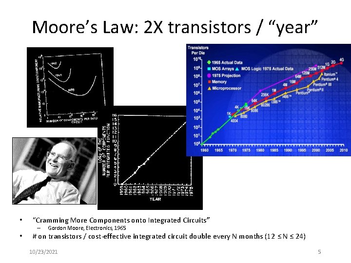
Moore’s Law: 2 X transistors / “year” • “Cramming More Components onto Integrated Circuits” – • Gordon Moore, Electronics, 1965 # on transistors / cost-effective integrated circuit double every N months (12 ≤ N ≤ 24) 10/23/2021 5

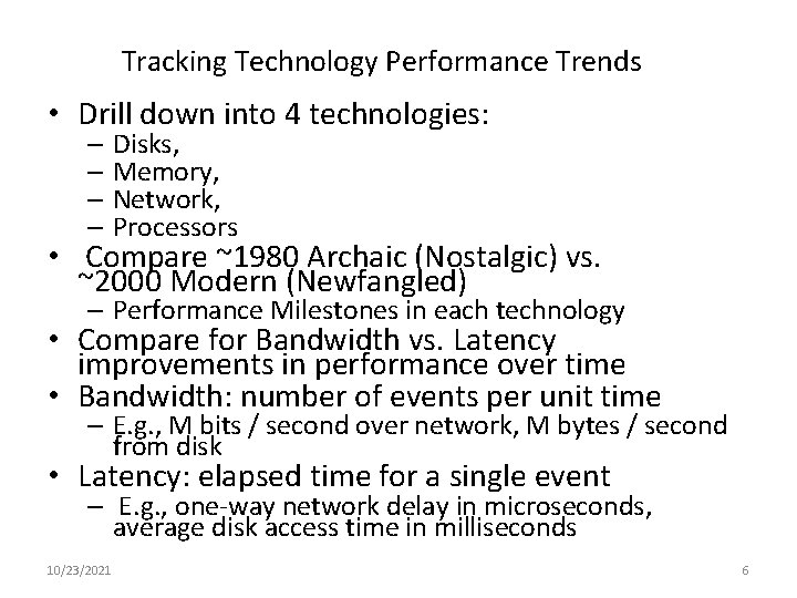
Tracking Technology Performance Trends • Drill down into 4 technologies: – Disks, – Memory, – Network, – Processors • Compare ~1980 Archaic (Nostalgic) vs. ~2000 Modern (Newfangled) – Performance Milestones in each technology • Compare for Bandwidth vs. Latency improvements in performance over time • Bandwidth: number of events per unit time – E. g. , M bits / second over network, M bytes / second from disk • Latency: elapsed time for a single event – E. g. , one-way network delay in microseconds, average disk access time in milliseconds 10/23/2021 6

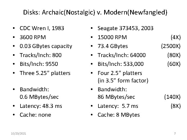
Disks: Archaic(Nostalgic) v. Modern(Newfangled) • • • CDC Wren I, 1983 3600 RPM 0. 03 GBytes capacity Tracks/Inch: 800 Bits/Inch: 9550 Three 5. 25” platters • Bandwidth: 0. 6 MBytes/sec • Latency: 48. 3 ms • Cache: none 10/23/2021 Seagate 373453, 2003 15000 RPM 73. 4 GBytes Tracks/Inch: 64000 Bits/Inch: 533, 000 Four 2. 5” platters (in 3. 5” form factor) • Bandwidth: 86 MBytes/sec • Latency: 5. 7 ms • Cache: 8 MBytes • • • (4 X) (2500 X) (80 X) (60 X) (140 X) (8 X) 7

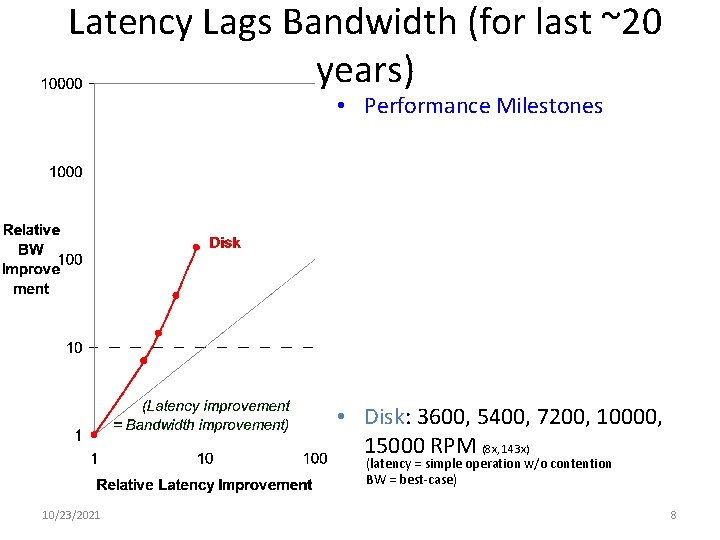
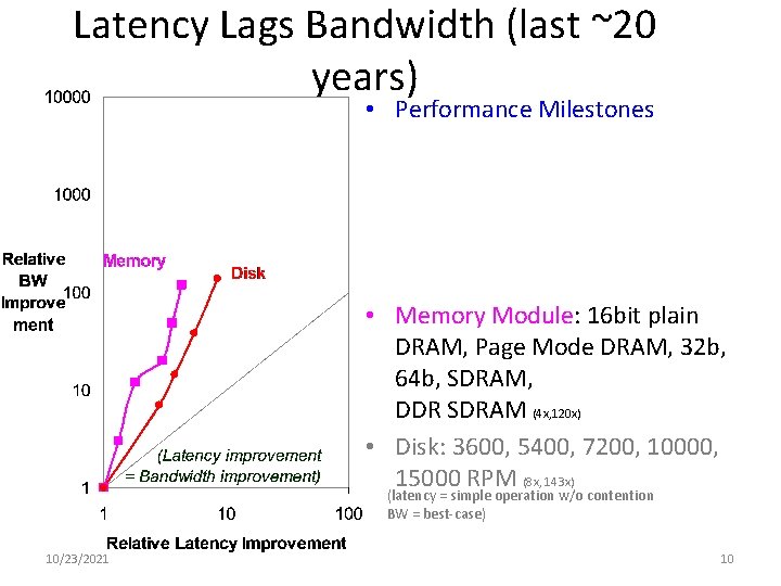
Latency Lags Bandwidth (for last ~20 years) • Performance Milestones • Disk: 3600, 5400, 7200, 10000, 15000 RPM (8 x, 143 x) (latency = simple operation w/o contention BW = best-case) 10/23/2021 8

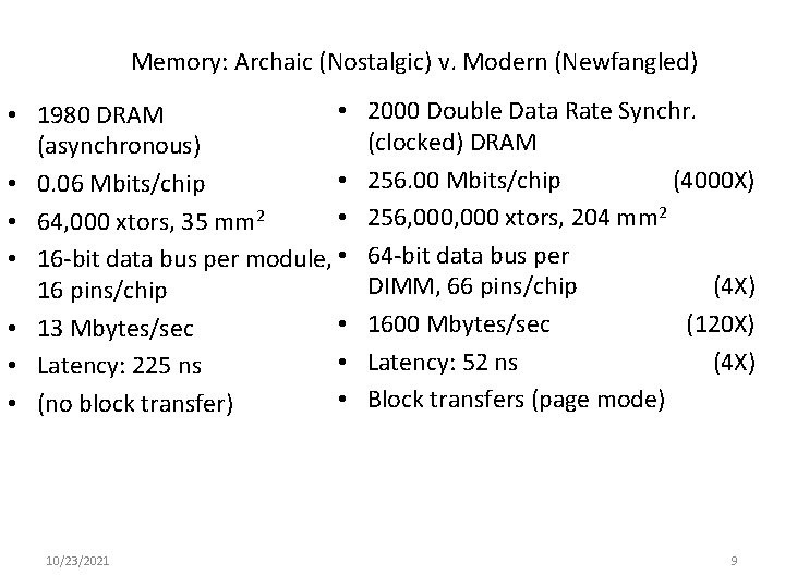
Memory: Archaic (Nostalgic) v. Modern (Newfangled) • • 1980 DRAM (asynchronous) • • 0. 06 Mbits/chip • • 64, 000 xtors, 35 mm 2 • 16 -bit data bus per module, • 16 pins/chip • • 13 Mbytes/sec • • Latency: 225 ns • • (no block transfer) 10/23/2021 2000 Double Data Rate Synchr. (clocked) DRAM 256. 00 Mbits/chip (4000 X) 256, 000 xtors, 204 mm 2 64 -bit data bus per DIMM, 66 pins/chip (4 X) 1600 Mbytes/sec (120 X) Latency: 52 ns (4 X) Block transfers (page mode) 9

Latency Lags Bandwidth (last ~20 years) • Performance Milestones • Memory Module: 16 bit plain DRAM, Page Mode DRAM, 32 b, 64 b, SDRAM, DDR SDRAM (4 x, 120 x) • Disk: 3600, 5400, 7200, 10000, 15000 RPM (8 x, 143 x) (latency = simple operation w/o contention BW = best-case) 10/23/2021 10

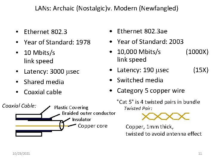
LANs: Archaic (Nostalgic)v. Modern (Newfangled) • Ethernet 802. 3 • Year of Standard: 1978 • 10 Mbits/s link speed • Latency: 3000 msec • Shared media • Coaxial cable Coaxial Cable: Plastic Covering Braided outer conductor Insulator Copper core 10/23/2021 • Ethernet 802. 3 ae • Year of Standard: 2003 • 10, 000 Mbits/s (1000 X) link speed • Latency: 190 msec (15 X) • Switched media • Category 5 copper wire "Cat 5" is 4 twisted pairs in bundle Twisted Pair: Copper, 1 mm thick, twisted to avoid antenna effect 11

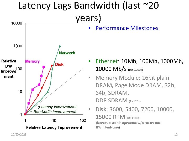
Latency Lags Bandwidth (last ~20 years) • Performance Milestones • Ethernet: 10 Mb, 1000 Mb, 10000 Mb/s (16 x, 1000 x) • Memory Module: 16 bit plain DRAM, Page Mode DRAM, 32 b, 64 b, SDRAM, DDR SDRAM (4 x, 120 x) • Disk: 3600, 5400, 7200, 10000, 15000 RPM (8 x, 143 x) (latency = simple operation w/o contention BW = best-case) 10/23/2021 12

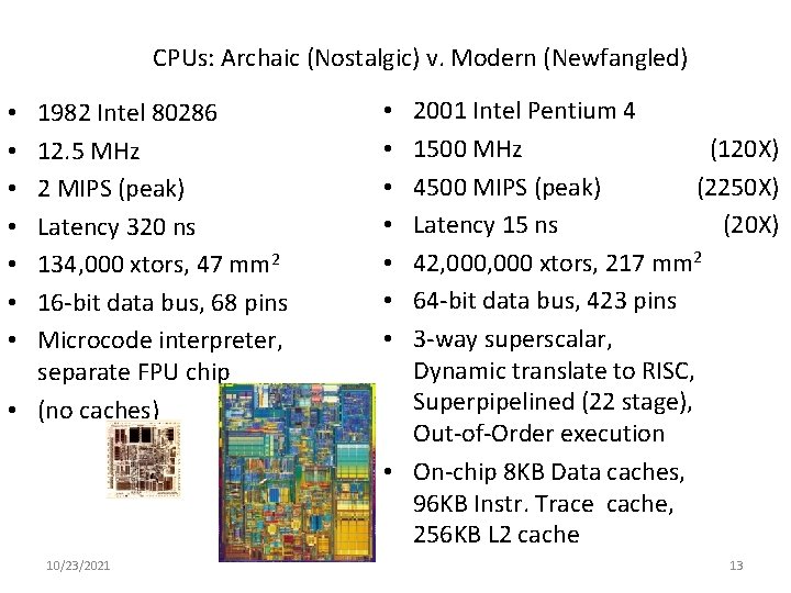
CPUs: Archaic (Nostalgic) v. Modern (Newfangled) 1982 Intel 80286 12. 5 MHz 2 MIPS (peak) Latency 320 ns 134, 000 xtors, 47 mm 2 16 -bit data bus, 68 pins Microcode interpreter, separate FPU chip • (no caches) • • 10/23/2021 2001 Intel Pentium 4 1500 MHz (120 X) 4500 MIPS (peak) (2250 X) Latency 15 ns (20 X) 42, 000 xtors, 217 mm 2 64 -bit data bus, 423 pins 3 -way superscalar, Dynamic translate to RISC, Superpipelined (22 stage), Out-of-Order execution • On-chip 8 KB Data caches, 96 KB Instr. Trace cache, 256 KB L 2 cache • • 13

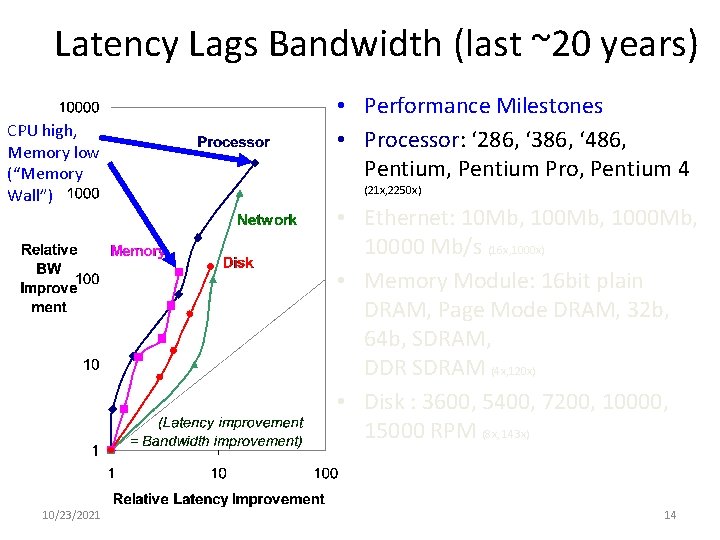
Latency Lags Bandwidth (last ~20 years) CPU high, Memory low (“Memory Wall”) 10/23/2021 • Performance Milestones • Processor: ‘ 286, ‘ 386, ‘ 486, Pentium Pro, Pentium 4 (21 x, 2250 x) • Ethernet: 10 Mb, 1000 Mb, 10000 Mb/s (16 x, 1000 x) • Memory Module: 16 bit plain DRAM, Page Mode DRAM, 32 b, 64 b, SDRAM, DDR SDRAM (4 x, 120 x) • Disk : 3600, 5400, 7200, 10000, 15000 RPM (8 x, 143 x) 14

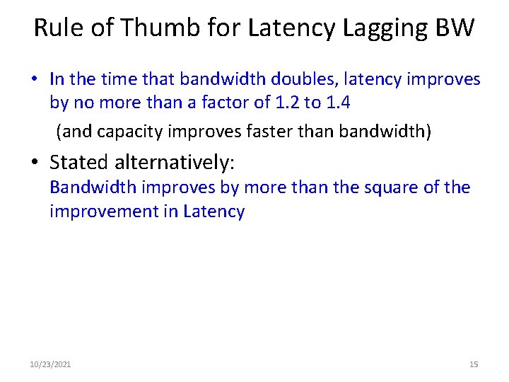
Rule of Thumb for Latency Lagging BW • In the time that bandwidth doubles, latency improves by no more than a factor of 1. 2 to 1. 4 (and capacity improves faster than bandwidth) • Stated alternatively: Bandwidth improves by more than the square of the improvement in Latency 10/23/2021 15

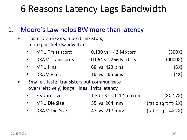
6 Reasons Latency Lags Bandwidth 1. Moore’s Law helps BW more than latency • • 10/23/2021 Faster transistors, more pins help Bandwidth • MPU Transistors: 0. 130 vs. 42 M xtors • DRAM Transistors: 0. 064 vs. 256 M xtors • MPU Pins: 68 vs. 423 pins • DRAM Pins: 16 vs. 66 pins Smaller, faster transistors but communicate over (relatively) longer lines: limits latency • Feature size: 1. 5 to 3 vs. 0. 18 micron • MPU Die Size: 35 vs. 204 mm 2 • DRAM Die Size: 47 vs. 217 mm 2 (300 X) (4000 X) (6 X) (4 X) (8 X, 17 X) (ratio sqrt 2 X) 16

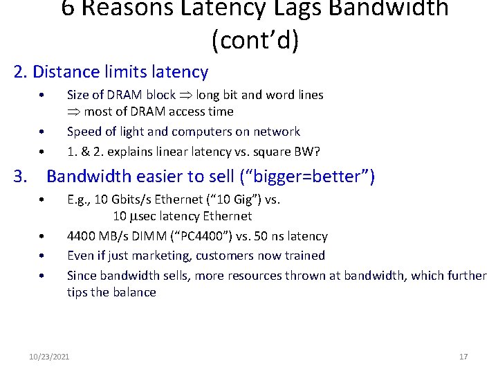
6 Reasons Latency Lags Bandwidth (cont’d) 2. Distance limits latency • • • Size of DRAM block long bit and word lines most of DRAM access time Speed of light and computers on network 1. & 2. explains linear latency vs. square BW? 3. Bandwidth easier to sell (“bigger=better”) • • E. g. , 10 Gbits/s Ethernet (“ 10 Gig”) vs. 10 msec latency Ethernet 4400 MB/s DIMM (“PC 4400”) vs. 50 ns latency Even if just marketing, customers now trained Since bandwidth sells, more resources thrown at bandwidth, which further tips the balance 10/23/2021 17

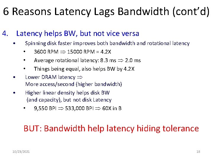
6 Reasons Latency Lags Bandwidth (cont’d) 4. Latency helps BW, but not vice versa • • • Spinning disk faster improves both bandwidth and rotational latency • 3600 RPM 15000 RPM = 4. 2 X • Average rotational latency: 8. 3 ms 2. 0 ms • Things being equal, also helps BW by 4. 2 X Lower DRAM latency More access/second (higher bandwidth) Higher linear density helps disk BW (and capacity), but not disk Latency • 9, 550 BPI 533, 000 BPI 60 X in B BUT: Bandwidth help latency hiding tolerance 10/23/2021 18

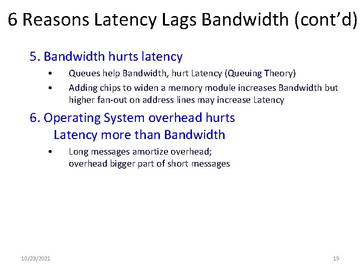
6 Reasons Latency Lags Bandwidth (cont’d) 5. Bandwidth hurts latency • • Queues help Bandwidth, hurt Latency (Queuing Theory) Adding chips to widen a memory module increases Bandwidth but higher fan-out on address lines may increase Latency 6. Operating System overhead hurts Latency more than Bandwidth • 10/23/2021 Long messages amortize overhead; overhead bigger part of short messages 19

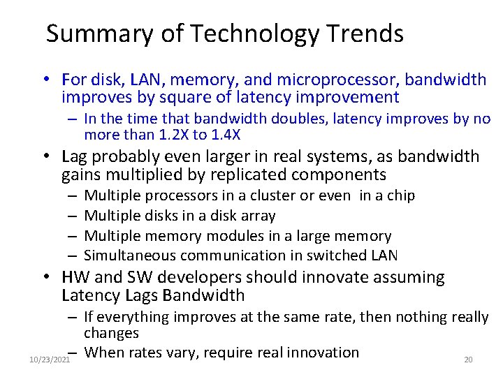
Summary of Technology Trends • For disk, LAN, memory, and microprocessor, bandwidth improves by square of latency improvement – In the time that bandwidth doubles, latency improves by no more than 1. 2 X to 1. 4 X • Lag probably even larger in real systems, as bandwidth gains multiplied by replicated components – – Multiple processors in a cluster or even in a chip Multiple disks in a disk array Multiple memory modules in a large memory Simultaneous communication in switched LAN • HW and SW developers should innovate assuming Latency Lags Bandwidth – If everything improves at the same rate, then nothing really changes – When rates vary, require real innovation 10/23/2021 20

Outline • Review • Technology Trends: Culture of tracking, anticipating and exploiting advances in technology • Careful, quantitative comparisons: 1. Define and quantity power 2. Define and quantity dependability 3. Define, quantity, and summarize relative performance 4. Define and quantity relative cost 10/23/2021 CS 252 -s 06, Lec 02 -intro 21

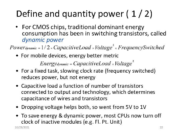
Define and quantity power ( 1 / 2) • For CMOS chips, traditional dominant energy consumption has been in switching transistors, called dynamic power • For mobile devices, energy better metric • For a fixed task, slowing clock rate (frequency switched) reduces power, but not energy • Capacitive load a function of number of transistors connected to output and technology, which determines capacitance of wires and transistors • Dropping voltage helps both, so went from 5 V to 1 V • To save energy & dynamic power, most CPUs now turn off clock of inactive modules (e. g. Fl. Pt. Unit) 10/23/2021 22

Example of quantifying power • Suppose 15% reduction in voltage results in a 15% reduction in frequency. What is impact on dynamic power? 10/23/2021 23

Define and quantity power (2 / 2) • Because leakage current flows even when a transistor is off, now static power important too • Leakage current increases in processors with smaller transistor sizes • Increasing the number of transistors increases power even if they are turned off • In 2006, goal for leakage is 25% of total power consumption; high performance designs at 40% • Very low power systems even gate voltage to inactive modules to control loss due to leakage 10/23/2021 24

Outline • Review • Technology Trends: Culture of tracking, anticipating and exploiting advances in technology • Careful, quantitative comparisons: 1. Define and quantity power 2. Define and quantity dependability 3. Define, quantity, and summarize relative performance 4. Define and quantity relative cost 10/23/2021 CS 252 -s 06, Lec 02 -intro 25

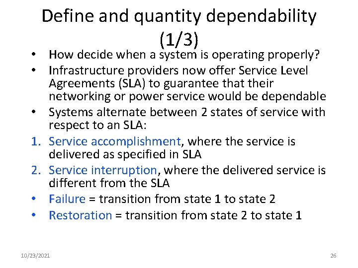
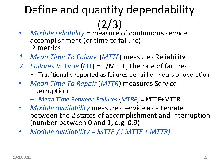
Define and quantity dependability (1/3) • How decide when a system is operating properly? • Infrastructure providers now offer Service Level Agreements (SLA) to guarantee that their networking or power service would be dependable • Systems alternate between 2 states of service with respect to an SLA: 1. Service accomplishment, where the service is delivered as specified in SLA 2. Service interruption, where the delivered service is different from the SLA • Failure = transition from state 1 to state 2 • Restoration = transition from state 2 to state 1 10/23/2021 26

Define and quantity dependability (2/3) Module reliability = measure of continuous service accomplishment (or time to failure). 2 metrics 1. Mean Time To Failure (MTTF) measures Reliability 2. Failures In Time (FIT) = 1/MTTF, the rate of failures • • Traditionally reported as failures per billion hours of operation • Mean Time To Repair (MTTR) measures Service Interruption – Mean Time Between Failures (MTBF) = MTTF+MTTR • • Module availability measures service as alternate between the 2 states of accomplishment and interruption (number between 0 and 1, e. g. 0. 9) Module availability = MTTF / ( MTTF + MTTR) 10/23/2021 27

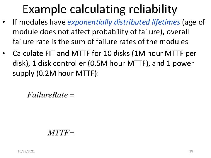
Example calculating reliability • If modules have exponentially distributed lifetimes (age of module does not affect probability of failure), overall failure rate is the sum of failure rates of the modules • Calculate FIT and MTTF for 10 disks (1 M hour MTTF per disk), 1 disk controller (0. 5 M hour MTTF), and 1 power supply (0. 2 M hour MTTF): 10/23/2021 28

Outline • Review • Technology Trends: Culture of tracking, anticipating and exploiting advances in technology • Careful, quantitative comparisons: 1. Define and quantity power 2. Define and quantity dependability 3. Define, quantity, and summarize relative performance 4. Define and quantity relative cost 10/23/2021 30

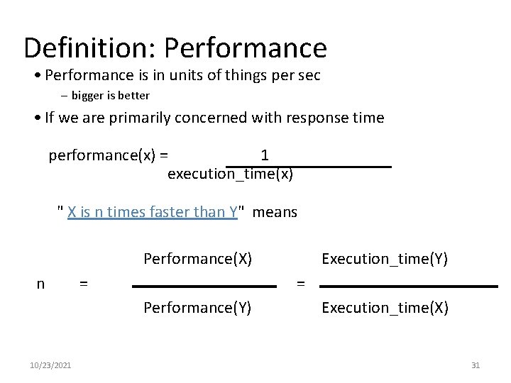
Definition: Performance • Performance is in units of things per sec – bigger is better • If we are primarily concerned with response time performance(x) = 1 execution_time(x) " X is n times faster than Y" means Performance(X) n = = Performance(Y) 10/23/2021 Execution_time(Y) Execution_time(X) 31

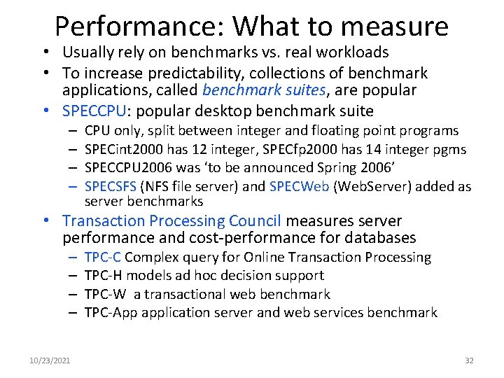
Performance: What to measure • Usually rely on benchmarks vs. real workloads • To increase predictability, collections of benchmark applications, called benchmark suites, are popular • SPECCPU: popular desktop benchmark suite – – CPU only, split between integer and floating point programs SPECint 2000 has 12 integer, SPECfp 2000 has 14 integer pgms SPECCPU 2006 was ‘to be announced Spring 2006’ SPECSFS (NFS file server) and SPECWeb (Web. Server) added as server benchmarks • Transaction Processing Council measures server performance and cost-performance for databases – – 10/23/2021 TPC-C Complex query for Online Transaction Processing TPC-H models ad hoc decision support TPC-W a transactional web benchmark TPC-App application server and web services benchmark 32

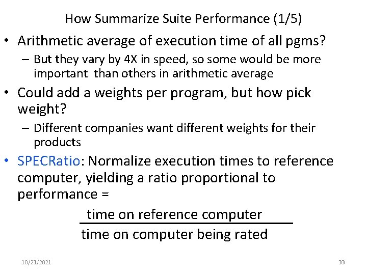
How Summarize Suite Performance (1/5) • Arithmetic average of execution time of all pgms? – But they vary by 4 X in speed, so some would be more important than others in arithmetic average • Could add a weights per program, but how pick weight? – Different companies want different weights for their products • SPECRatio: Normalize execution times to reference computer, yielding a ratio proportional to performance = time on reference computer time on computer being rated 10/23/2021 33

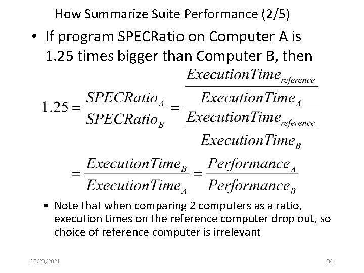
How Summarize Suite Performance (2/5) • If program SPECRatio on Computer A is 1. 25 times bigger than Computer B, then • Note that when comparing 2 computers as a ratio, execution times on the reference computer drop out, so choice of reference computer is irrelevant 10/23/2021 34

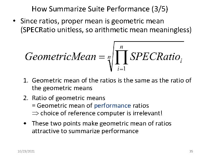
How Summarize Suite Performance (3/5) • Since ratios, proper mean is geometric mean (SPECRatio unitless, so arithmetic meaningless) 1. Geometric mean of the ratios is the same as the ratio of the geometric means 2. Ratio of geometric means = Geometric mean of performance ratios choice of reference computer is irrelevant! • These two points make geometric mean of ratios attractive to summarize performance 10/23/2021 35

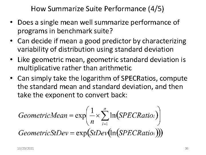
How Summarize Suite Performance (4/5) • Does a single mean well summarize performance of programs in benchmark suite? • Can decide if mean a good predictor by characterizing variability of distribution using standard deviation • Like geometric mean, geometric standard deviation is multiplicative rather than arithmetic • Can simply take the logarithm of SPECRatios, compute the standard mean and standard deviation, and then take the exponent to convert back: 10/23/2021 36

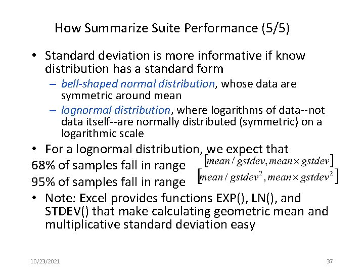
How Summarize Suite Performance (5/5) • Standard deviation is more informative if know distribution has a standard form – bell-shaped normal distribution, whose data are symmetric around mean – lognormal distribution, where logarithms of data--not data itself--are normally distributed (symmetric) on a logarithmic scale • For a lognormal distribution, we expect that 68% of samples fall in range 95% of samples fall in range • Note: Excel provides functions EXP(), LN(), and STDEV() that make calculating geometric mean and multiplicative standard deviation easy 10/23/2021 37

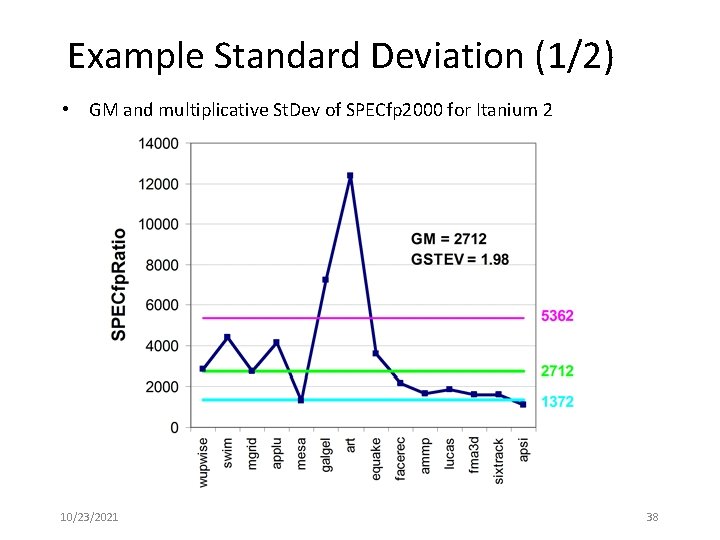
Example Standard Deviation (1/2) • GM and multiplicative St. Dev of SPECfp 2000 for Itanium 2 10/23/2021 38

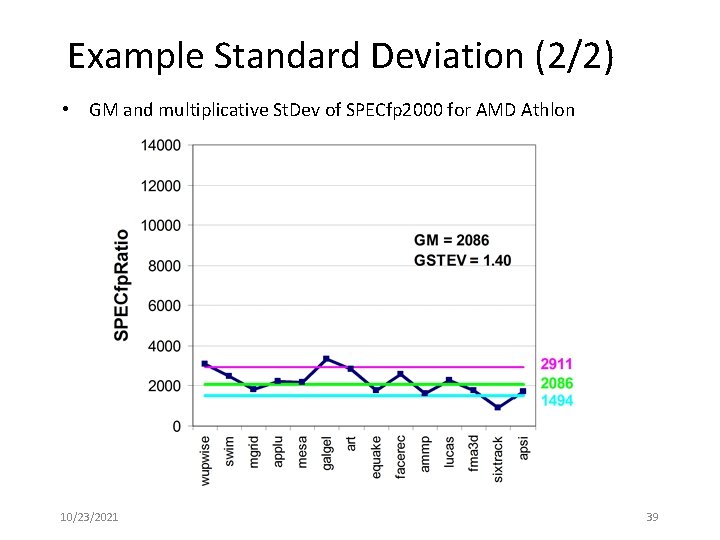
Example Standard Deviation (2/2) • GM and multiplicative St. Dev of SPECfp 2000 for AMD Athlon 10/23/2021 39

And in conclusion … • Tracking and extrapolating technology part of architect’s responsibility • Expect Bandwidth in disks, DRAM, network, and processors to improve by at least as much as the square of the improvement in Latency • Quantify dynamic and static power – Capacitance x Voltage 2 x frequency, Energy vs. power • Quantify dependability – Reliability (MTTF, FIT), Availability (99. 9…) • Quantify and summarize performance – Ratios, Geometric Mean, Multiplicative Standard Deviation • Read Appendix A 10/23/2021 40