Comparing More Than Two Means Chapter 9 Review

Comparing More Than Two Means Chapter 9

Review of Simulation-Based Tests • One proportion: • We created a null distribution by flipping a coin, rolling a die, or some computer simulation. • We then found where our sample proportion was in this null distribution.

Simulation-Based Tests • Comparing two proportions: • Assuming there was no association between explanatory and response variables (the difference in proportions is zero), we shuffled cards and dealt them into two piles. (This essentially scrambled the response variable. ) • We then calculated the difference in proportions. • We repeated this process many times and built a null distribution. • We finally found where the observed difference in sample proportions was located in the null distribution.

Simulation-Based Tests • Comparing two means: • Assuming there was no association between explanatory and response variables (the difference in means is zero), we shuffled cards and dealt them into two piles. (This time the cards had numbers on them, the response, instead of words) • We then calculated the difference in means • We repeated this process many times and built a null distribution. • We finally found where the observed difference in sample means was located in the null distribution.

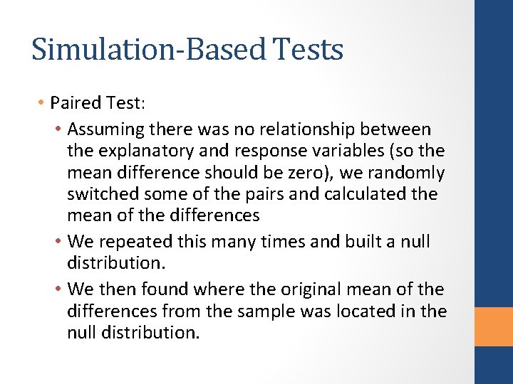
Simulation-Based Tests • Paired Test: • Assuming there was no relationship between the explanatory and response variables (so the mean difference should be zero), we randomly switched some of the pairs and calculated the mean of the differences • We repeated this many times and built a null distribution. • We then found where the original mean of the differences from the sample was located in the null distribution.

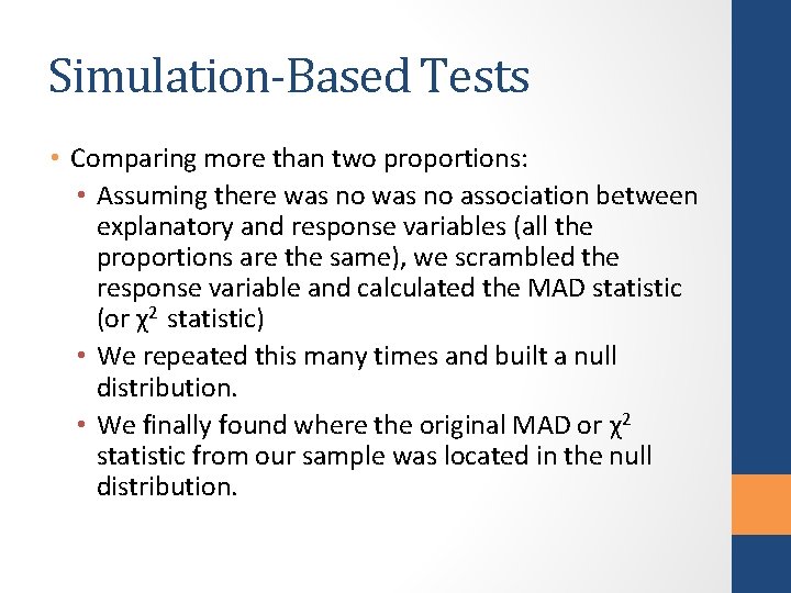
Simulation-Based Tests • Comparing more than two proportions: • Assuming there was no association between explanatory and response variables (all the proportions are the same), we scrambled the response variable and calculated the MAD statistic (or χ2 statistic) • We repeated this many times and built a null distribution. • We finally found where the original MAD or χ2 statistic from our sample was located in the null distribution.

Two more types of tests • We now want to compare multiple (more than two) means. • In chapter 10 we will look at an association between two quantitative variables using correlation and regression. • Both of these processes are basically the same as most of the simulation-based tests we have already done. Just the data types (or number of categories) and the statistic we use is different.

Follow up tests • In the last chapter, we tested multiple proportions and if we found significance, we followed this up with by calculating confidence intervals to find out exactly which proportions were different. • Why didn’t we just start out finding a number of confidence intervals? • Let’s go through the following example to answer this and introduce tests for multiple means.

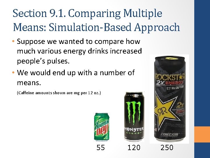
Section 9. 1. Comparing Multiple Means: Simulation-Based Approach • Suppose we wanted to compare how much various energy drinks increased people’s pulses. • We would end up with a number of means. (Caffeine amounts shown are mg per 12 oz. ) 55 120 250

Controlling for Type I Error • We could do this with multiple tests where we compared two means at a time, but • If we were comparing 3 means, we would have to use 3 two-sample tests to compare these three means. (A vs B, B vs C, and A vs C) • If each test has a 5% significance level, there’s a 5% chance making a Type I Error. • Remember we can call this a false alarm. • Rejecting the null when it is true. • There really is no difference between our groups and we got a result out in the tail just by chance alone.

Controlling for Type I Error • These type I errors “accumulate” when we do more tests on the same data. • At the 5% significance level, the probability of making at least one type I error for three test would be 14%. • Comparing 4 means (6 tests), this jumps to 26%. • Comparing 5 means (10 tests), this jumps to 40%. • An alternative approach uses one over-all test that compares all means at once.

Overall Test • We used one overall test in the last chapter when we compared proportions and we will do the same for comparing means. • If I have two means to compare, we just need to look at their difference to measure how far apart they are. • Suppose we wanted to compare three means. How could I create something that would measure how different all three means are?

MAD Statistic • We will use the same MAD statistic as before, but this time look at the mean absolute differences for averages. • MAD = (|avg 1 – avg 2|+|avg 2 – avg 3|+ |avg 2 – avg 3|)/3 • Let’s try this on an example! (Don’t follow along in your book or look ahead on the Power. Point. )

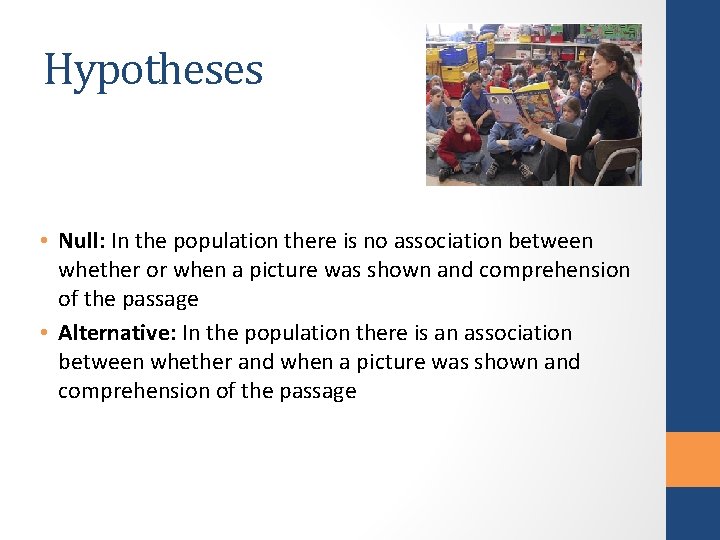
Comprehension Example • Students were read an ambiguous prose passage under one of the following conditions: • Students were given a picture that could help them interpret the passage before they heard it. • Students were given the picture after they heard the passage. • Students were not shown any picture before or after hearing the passage. • They were then asked to evaluate their comprehension of the passage on a 1 to 7 scale.

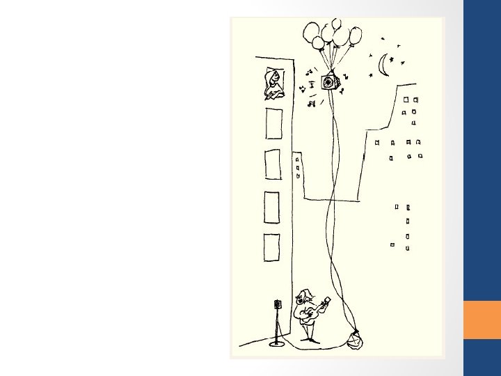
Comprehension Example • This experiment is a partial replication done here at Hope of a study done by Bransford and Johnson (1972). • The students were randomly assigned to one of the three groups. • Let’s listen to the passage and see if it makes sense. • Would a picture help?

Hypotheses • Null: In the population there is no association between whether or when a picture was shown and comprehension of the passage • Alternative: In the population there is an association between whether and when a picture was shown and comprehension of the passage

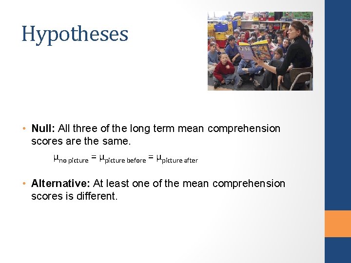
Hypotheses • Null: All three of the long term mean comprehension scores are the same. µno picture = µpicture before = µpicture after • Alternative: At least one of the mean comprehension scores is different.

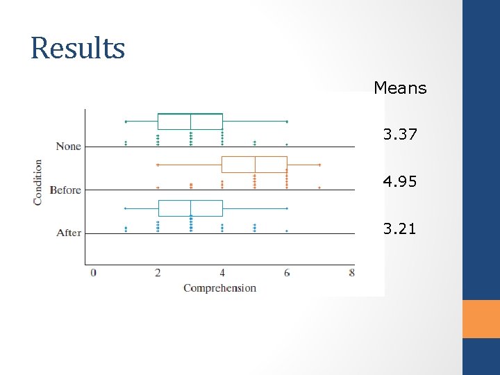
Results Means 3. 37 4. 95 3. 21

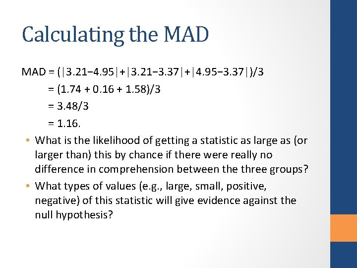
Calculating the MAD = (|3. 21− 4. 95|+|3. 21− 3. 37|+|4. 95− 3. 37|)/3 = (1. 74 + 0. 16 + 1. 58)/3 = 3. 48/3 = 1. 16. • What is the likelihood of getting a statistic as large as (or larger than) this by chance if there were really no difference in comprehension between the three groups? • What types of values (e. g. , large, small, positive, negative) of this statistic will give evidence against the null hypothesis?

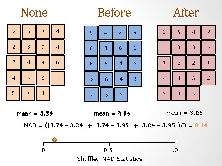
Simulation • Similar to testing two means we can shuffle values of the response variable (the comprehension scores) and randomly place them into piles representing the categories of the explanatory variable (the picture condition). • This time we have three piles instead of two. • After each shuffle, we calculate the MAD statistic of the shuffled data and that will be a point in the null distribution.

None Before After 2 5 3 4 5 4 2 6 6 5 4 2 2 3 2 4 6 3 6 6 1 3 3 5 2 4 4 6 6 5 4 6 3 2 2 1 4 3 3 1 5 6 4 3 4 4 3 2 5 3 4 7 5 5 5 3 3 mean = 3. 74 mean = 3. 37 mean = 3. 84 mean = 4. 95 mean = 3. 21 mean = 3. 95 MAD = (|3. 74 – 3. 84| + |3. 74 – 3. 95| + |3. 84 – 3. 95|)/3 = 0. 14 0 0. 5 1. 0 Shuffled MAD Statistics

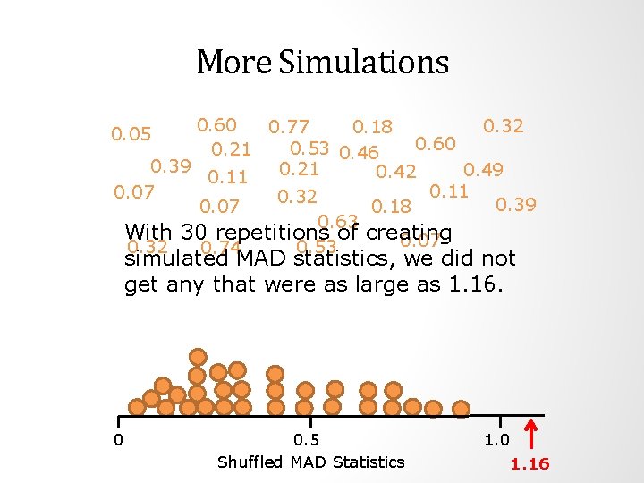
More Simulations 0. 60 0. 32 0. 77 0. 18 0. 60 0. 53 0. 46 0. 21 0. 39 0. 21 0. 49 0. 42 0. 11 0. 07 0. 32 0. 39 0. 18 0. 07 0. 63 With 30 repetitions of creating 0. 07 0. 53 0. 32 0. 74 0. 05 simulated MAD statistics, we did not get any that were as large as 1. 16. 0 0. 5 1. 0 Shuffled MAD Statistics 1. 16

Let’s test this • Get the data from the website. • Go to the Multiple Means Applet and paste in the data. • Run the test. This applet is the same one we used in chapter 6 when we compared two means.

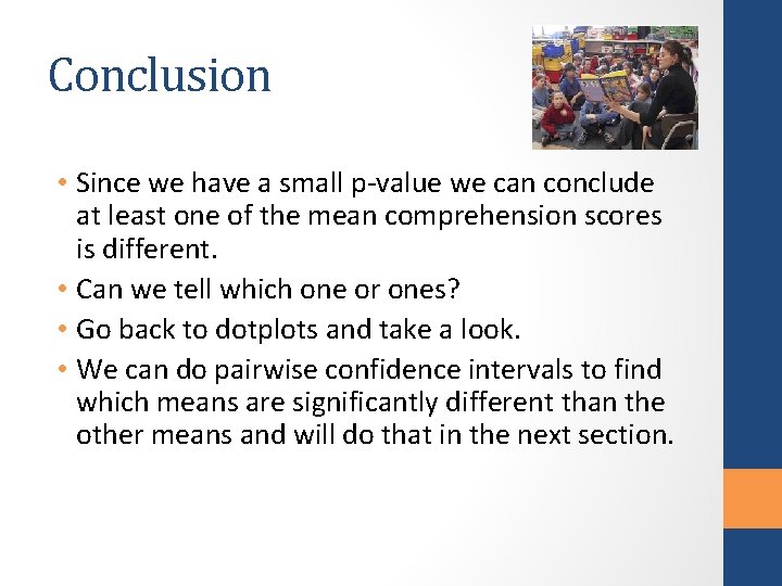
Conclusion • Since we have a small p-value we can conclude at least one of the mean comprehension scores is different. • Can we tell which one or ones? • Go back to dotplots and take a look. • We can do pairwise confidence intervals to find which means are significantly different than the other means and will do that in the next section.

Learning Objectives for Section 9. 1 • Be able to calculate the MAD statistic given a data set (or set of means). • Understand how a simulation-based test would work using cards and shuffling for comparing multiple means. • Understand that we do an overall test when comparing multiple means or proportions instead of pairwise tests to control for the probability of making a type I error. • Use the multiple means applet to carry out an analysis using the MAD statistic to compare multiple means.

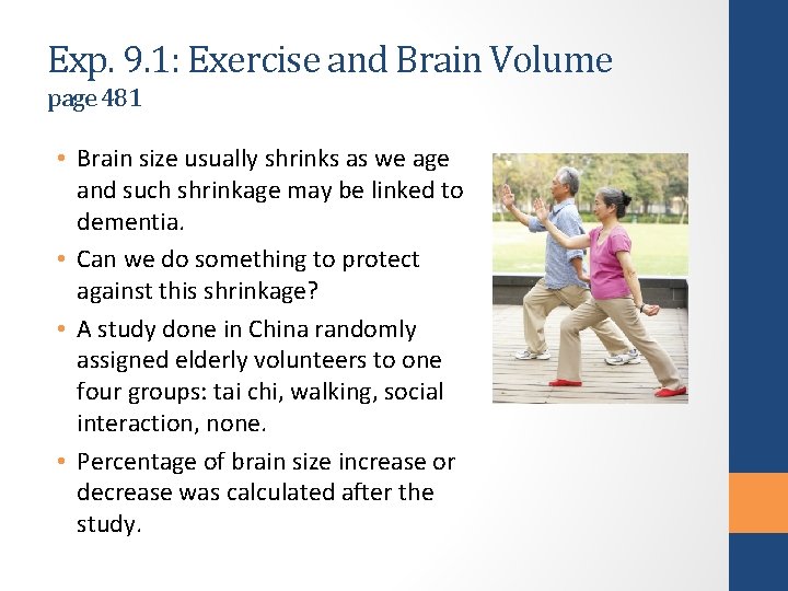
Exp. 9. 1: Exercise and Brain Volume page 481 • Brain size usually shrinks as we age and such shrinkage may be linked to dementia. • Can we do something to protect against this shrinkage? • A study done in China randomly assigned elderly volunteers to one four groups: tai chi, walking, social interaction, none. • Percentage of brain size increase or decrease was calculated after the study.

Comparing Multiple Means: Theory-Based Approach (ANalysis Of Variance ANOVA) Section 9. 2

ANOVA • Like in chapter 8 when we compared multiple proportions, we need a statistic other than the MAD to make the transition to theory-based a smooth one. • This new statistic is called an F statistic and theory-based distribution that estimates our null distribution is called an F distribution. • Unlike the MAD statistic, the F statistic takes into account the variability within each group.

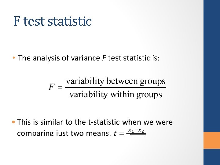
F test statistic • The analysis of variance F test statistic is:

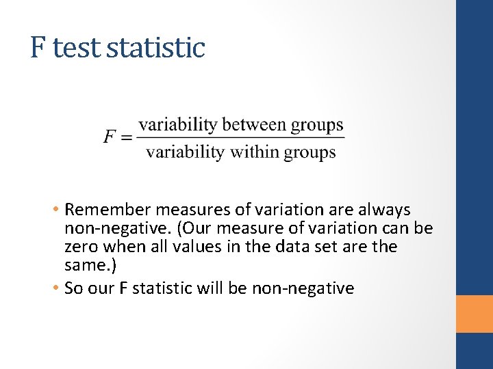
F test statistic • Remember measures of variation are always non-negative. (Our measure of variation can be zero when all values in the data set are the same. ) • So our F statistic will be non-negative

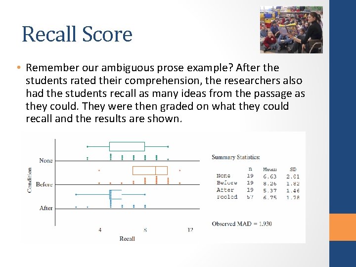
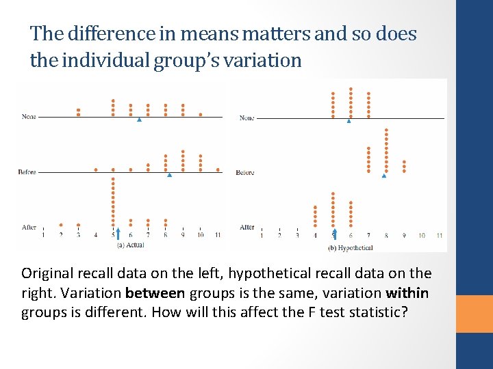
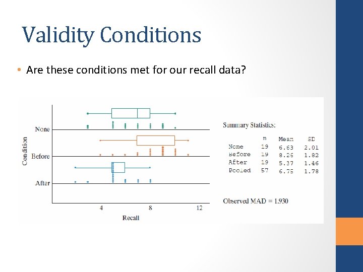
Recall Score • Remember our ambiguous prose example? After the students rated their comprehension, the researchers also had the students recall as many ideas from the passage as they could. They were then graded on what they could recall and the results are shown.

The difference in means matters and so does the individual group’s variation Original recall data on the left, hypothetical recall data on the right. Variation between groups is the same, variation within groups is different. How will this affect the F test statistic?

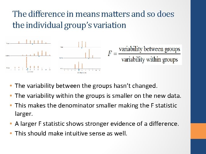
The difference in means matters and so does the individual group’s variation • The variability between the groups hasn’t changed. • The variability within the groups is smaller on the new data. • This makes the denominator smaller making the F statistic larger. • A larger F statistic shows stronger evidence of a difference. • This should make intuitive sense as well.

Hypotheses • Null: All three of the long-run mean recall scores for students under the different conditions are the same. (No association) • Alternative: At least one of the long-run mean recall scores for students under the different conditions is different. (Association)

Validity Conditions • Just as with the simulation-based method, we are assuming we have independent groups. • Two extra conditions must be met to use traditional ANOVA: • Normality: If sample sizes are small within each group, data shouldn’t be very skewed. If it is, use simulation approach. (samples sizes of 20 again is a good guideline for means) • Equal variation: Largest standard deviation is not more than twice the value of the smallest.

Validity Conditions • Are these conditions met for our recall data?

Let’s run the ANOVA test • Let’s get the Recall data and run the test using the same applet we used last time (Multiple Means Applet) • Let’s do simulation using the MAD statistic as well as the F statistic. • Then do theory-based methods using ANOVA. • If we get a small p-value, we will follow this overall test up with confidence intervals to determine exactly where the difference occurs.

Conclusion • Since we have a small p-value we have strong evidence against the null and can conclude at least one of the long -run mean recall scores is different. • From our confidence intervals, • After - Before: (-4. 05, -1. 74)* • After - None: (-2. 42, -0. 11)* • Before - None: (0. 4756, 2. 7875)* • We can see that each is significant so • µpicture after ≠ µpicture before • µpictureafter ≠ µno picture • µpicture before ≠ µno picture

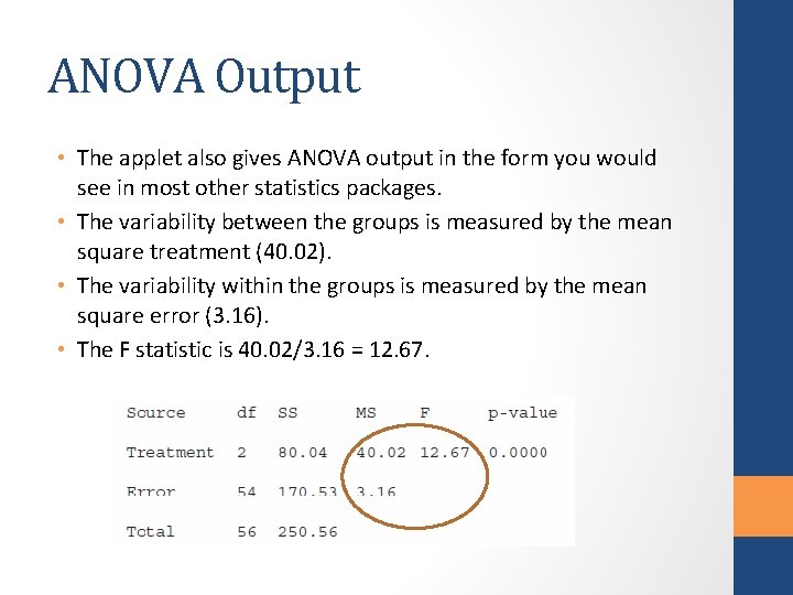
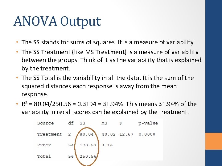
ANOVA Output • The applet also gives ANOVA output in the form you would see in most other statistics packages. • The variability between the groups is measured by the mean square treatment (40. 02). • The variability within the groups is measured by the mean square error (3. 16). • The F statistic is 40. 02/3. 16 = 12. 67.

ANOVA Output • The SS stands for sums of squares. It is a measure of variability. • The SS Treatment (like MS Treatment) is a measure of variability between the groups. Think of it as the variability that is explained by the treatment. • The SS Total is the variability in all the data. It is the sum of the squared distances each response is away from the mean response. • R 2 = 80. 04/250. 56 = 0. 3194 = 31. 94%. This means 31. 94% of the variability in recall scores can be explained by the treatment.

Strength of Evidence • As sample size increases, strength of evidence increases. • As the means move farther apart, strength of evidence increases. (This is the variability between groups. ) • As the standard deviations increase, strength of evidence decreases. (This is the variability within groups. ) • These are all exactly the same as when we compared two means.

Learning Objectives for Section 9. 2 • Find the value of the F statistic using the multiple means applet, recognize that larger values of the statistic mean more evidence against the null hypothesis and that the distribution of the F statistic is positive and skewed right. • Identify whether or not an ANOVA (F) test meets appropriate validity conditions. • Conduct an ANOVA using the multiple means applet, including appropriate follow-up tests.

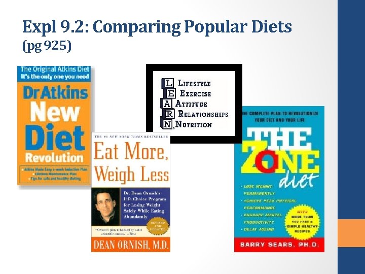
Expl 9. 2: Comparing Popular Diets (pg 925)

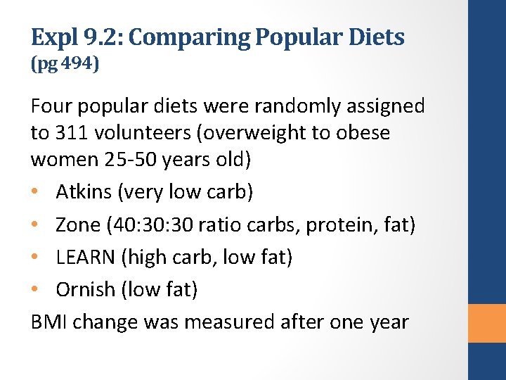
Expl 9. 2: Comparing Popular Diets (pg 494) Four popular diets were randomly assigned to 311 volunteers (overweight to obese women 25 -50 years old) • Atkins (very low carb) • Zone (40: 30 ratio carbs, protein, fat) • LEARN (high carb, low fat) • Ornish (low fat) BMI change was measured after one year