Collocations Many slides from Rada Mihalcea Michigan Paul

Collocations Many slides from Rada Mihalcea (Michigan), Paul Tarau (U. North Texas)

Outline • • What is a collocation? Automatic approaches 1: frequency-based methods Automatic approaches 2: ruling out the null hypothesis, t-test Automatic approaches 3: chi-square and mutual information

Criteria for Collocations • Typical criteria for collocations: – non-compositionality – non-substitutability – non-modifiability. • Collocations usually cannot be translated into other languages word by word. • A phrase can be a collocation even if it is not consecutive (as in the example knock. . . door).

Non-Compositionality • A phrase is compositional if the meaning can be predicted from the meaning of the parts. – E. g. , new companies • A phrase is non-compositional if the meaning cannot be predicted from the meaning of the parts – E. g. , hot dog • Collocations are not necessarily fully compositional in that there is usually an element of meaning added to the combination. Eg. , strong tea. • Idioms are the most extreme examples of non-compositionality. Eg. , to hear it through the grapevine.

Non-Substitutability • We cannot substitute near-synonyms for the components of a collocation. • For example – We can’t say yellow wine instead of white wine even though yellow is as good a description of the color of white wine as white is (it is kind of a yellowish white). • Many collocations cannot be freely modified with additional lexical material or through grammatical transformations (Nonmodifiability). – E. g. , white wine, but not whiter wine – mother in law, but not mother in laws (it would be mothers in law)

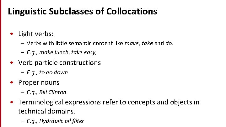
Linguistic Subclasses of Collocations • Light verbs: – Verbs with little semantic content like make, take and do. – E. g. , make lunch, take easy, • Verb particle constructions – E. g. , to go down • Proper nouns – E. g. , Bill Clinton • Terminological expressions refer to concepts and objects in technical domains. – E. g. , Hydraulic oil filter

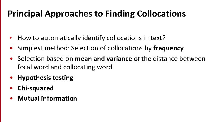
Principal Approaches to Finding Collocations • How to automatically identify collocations in text? • Simplest method: Selection of collocations by frequency • Selection based on mean and variance of the distance between focal word and collocating word • Hypothesis testing • Chi-squared • Mutual information

Outline • • What is a collocation? Automatic approaches 1: frequency-based methods Automatic approaches 2: ruling out the null hypothesis, t-test Automatic approaches 3: chi-square and mutual information

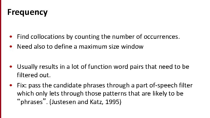
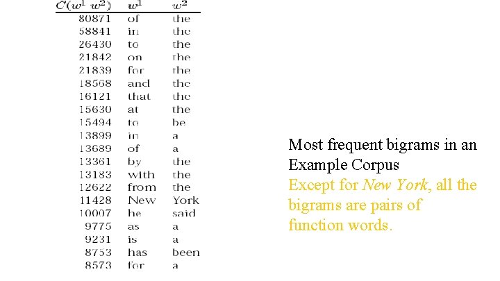
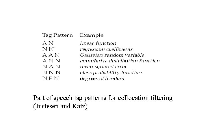
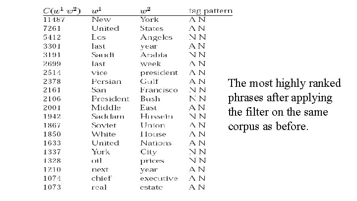
Frequency • Find collocations by counting the number of occurrences. • Need also to define a maximum size window • Usually results in a lot of function word pairs that need to be filtered out. • Fix: pass the candidate phrases through a part of-speech filter which only lets through those patterns that are likely to be “phrases”. (Justesen and Katz, 1995)

Most frequent bigrams in an Example Corpus Except for New York, all the bigrams are pairs of function words.

Part of speech tag patterns for collocation filtering (Justesen and Katz).

The most highly ranked phrases after applying the filter on the same corpus as before.

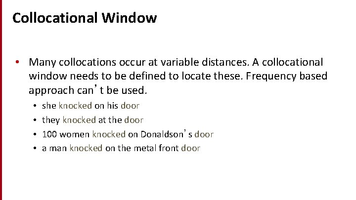
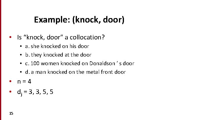
Collocational Window • Many collocations occur at variable distances. A collocational window needs to be defined to locate these. Frequency based approach can’t be used. • • she knocked on his door they knocked at the door 100 women knocked on Donaldson’s door a man knocked on the metal front door

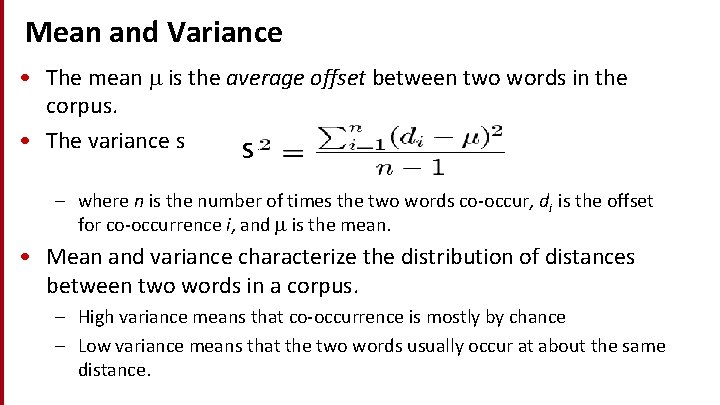
Mean and Variance • The mean is the average offset between two words in the corpus. • The variance s s – where n is the number of times the two words co-occur, di is the offset for co-occurrence i, and is the mean. • Mean and variance characterize the distribution of distances between two words in a corpus. – High variance means that co-occurrence is mostly by chance – Low variance means that the two words usually occur at about the same distance.

Example: (knock, door) • Is “knock, door” a collocation? • • a. she knocked on his door b. they knocked at the door c. 100 women knocked on Donaldson ’ s door d. a man knocked on the metal front door • n=4 • dj = 3, 3, 5, 5 15

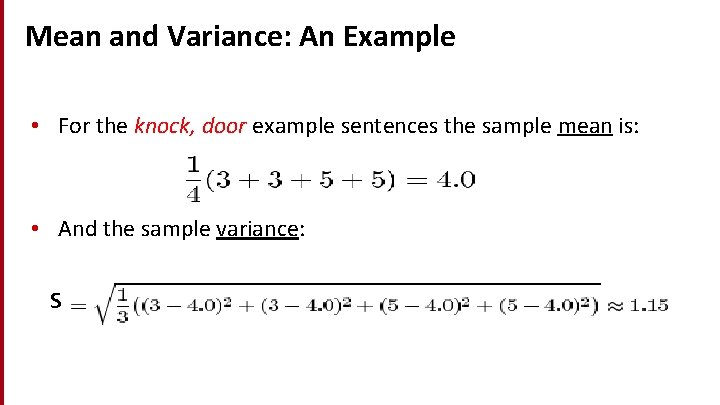
Mean and Variance: An Example • For the knock, door example sentences the sample mean is: • And the sample variance: s

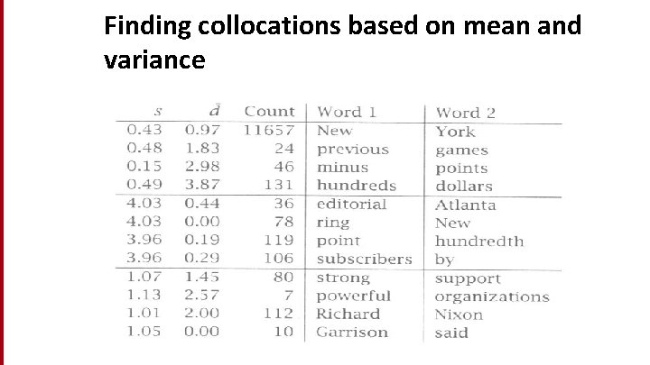
Finding collocations based on mean and variance

Outline • • What is a collocation? Automatic approaches 1: frequency-based methods Automatic approaches 2: ruling out the null hypothesis, t-test Automatic approaches 3: chi-square and mutual information

Ruling out Chance • Two words can co-occur by chance. – High frequency and low variance can be accidental • Hypothesis Testing measures the confidence that this cooccurrence was really due to association, and not just due to chance. • Formulate a null hypothesis H 0 that there is no association between the words beyond chance occurrences. • The null hypothesis states what should be true if two words do not form a collocation. • i. e. , H 0: The two words occur together by chance (randomness).

Ruling out Chance (cont’d) • If the null hypothesis can be rejected, then the two words do not co-occur by chance, and they form a collocation • Compute the probability p that the event would occur if H 0 were true, and then reject H 0 if p is too low (typically if beneath a significance level of p < 0. 05, 0. 01, 0. 005, or 0. 001) and retain H 0 as possible otherwise. 20

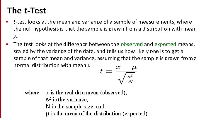
The t-Test • t-test looks at the mean and variance of a sample of measurements, where the null hypothesis is that the sample is drawn from a distribution with mean . • The test looks at the difference between the observed and expected means, scaled by the variance of the data, and tells us how likely one is to get a sample of that mean and variance, assuming that the sample is drawn from a normal distribution with mean . where x is the real data mean (observed), s 2 is the variance, N is the sample size, and is the mean of the distribution (expected).

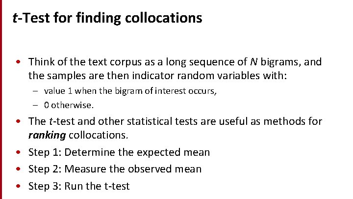
t-Test for finding collocations • Think of the text corpus as a long sequence of N bigrams, and the samples are then indicator random variables with: – value 1 when the bigram of interest occurs, – 0 otherwise. • The t-test and other statistical tests are useful as methods for ranking collocations. • Step 1: Determine the expected mean • Step 2: Measure the observed mean • Step 3: Run the t-test

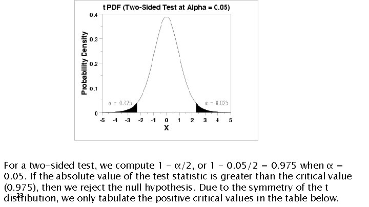
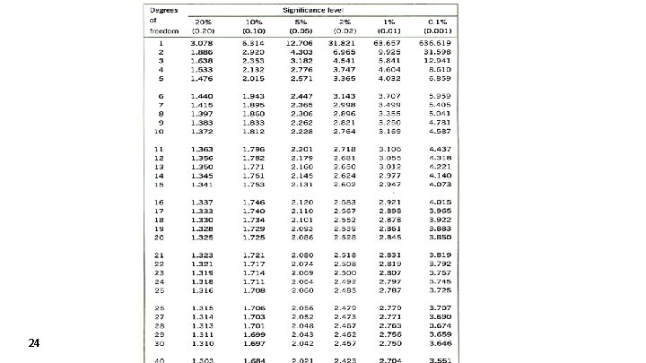
For a two-sided test, we compute 1 - α/2, or 1 - 0. 05/2 = 0. 975 when α = 0. 05. If the absolute value of the test statistic is greater than the critical value (0. 975), then we reject the null hypothesis. Due to the symmetry of the t 23 distribution, we only tabulate the positive critical values in the table below.

24

Degrees of freedom number of samples -1 i. e. , n-1 25

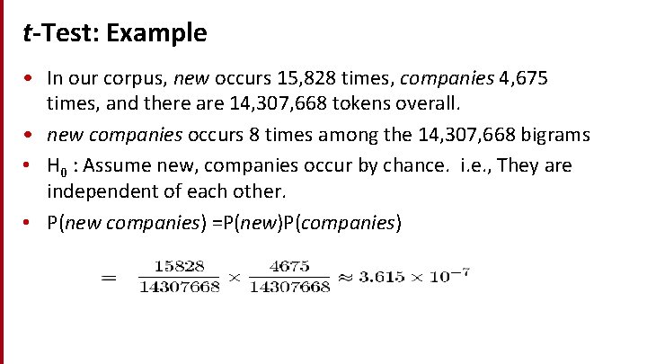
t-Test: Example • In our corpus, new occurs 15, 828 times, companies 4, 675 times, and there are 14, 307, 668 tokens overall. • new companies occurs 8 times among the 14, 307, 668 bigrams • H 0 : Assume new, companies occur by chance. i. e. , They are independent of each other. • P(new companies) =P(new)P(companies)

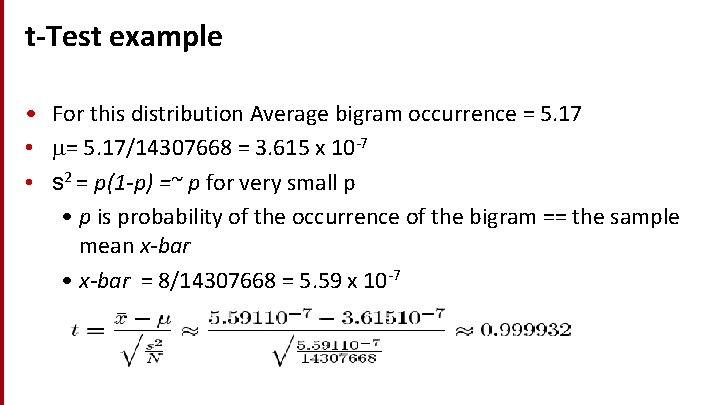
t-Test example • For this distribution Average bigram occurrence = 5. 17 • = 5. 17/14307668 = 3. 615 x 10 -7 • s 2 = p(1 -p) =~ p for very small p • p is probability of the occurrence of the bigram == the sample mean x-bar • x-bar = 8/14307668 = 5. 59 x 10 -7

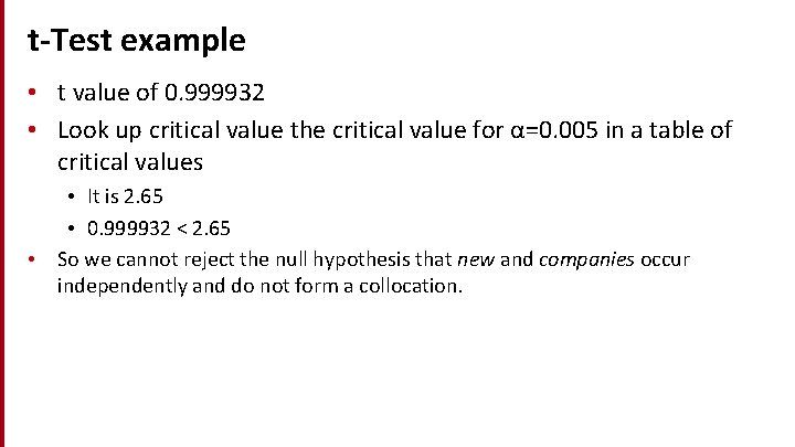
t-Test example • t value of 0. 999932 • Look up critical value the critical value for α=0. 005 in a table of critical values • It is 2. 65 • 0. 999932 < 2. 65 • So we cannot reject the null hypothesis that new and companies occur independently and do not form a collocation.

Outline • • What is a collocation? Automatic approaches 1: frequency-based methods Automatic approaches 2: ruling out the null hypothesis, t-test Automatic approaches 3: chi-square and mutual information

Pearson’s 2 (chi-square) test • t-test assumes that probabilities are approximately normally distributed, which is not true in general. The 2 test doesn’t make this assumption. • the essence of the 2 test is to compare the observed frequencies with the frequencies expected for independence – if the difference between observed and expected frequencies is large, then we can reject the null hypothesis of independence.

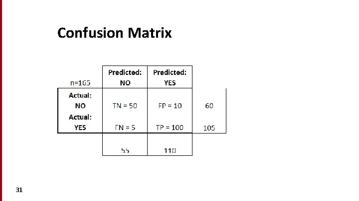
Confusion Matrix 31

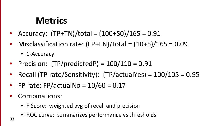
Metrics • Accuracy: (TP+TN)/total = (100+50)/165 = 0. 91 • Misclassification rate: (FP+FN)/total = (10+5)/165 = 0. 09 • 1 -Accuracy • • 32 Precision: (TP/predicted. P) = 100/110 = 0. 91 Recall (TP rate/Sensitivity): (TP/actual. Yes) = 100/105 = 0. 95 FP rate: FP/actual. No = 10/60 = 0. 17 Combinations: • F Score: weighted avg of recall and precision • ROC curve: summarizes performance vs thresholds

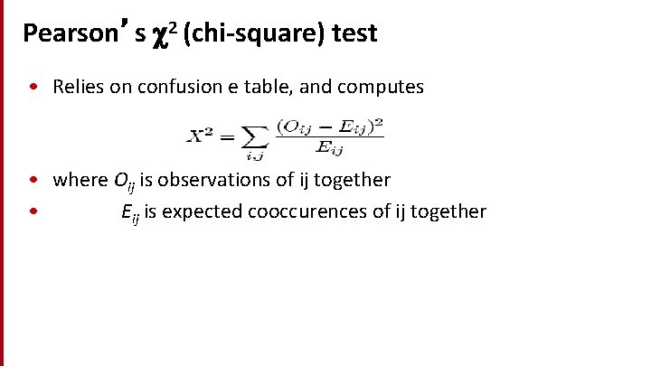
Pearson’s 2 (chi-square) test • Relies on confusion e table, and computes • where Oij is observations of ij together • Eij is expected cooccurences of ij together

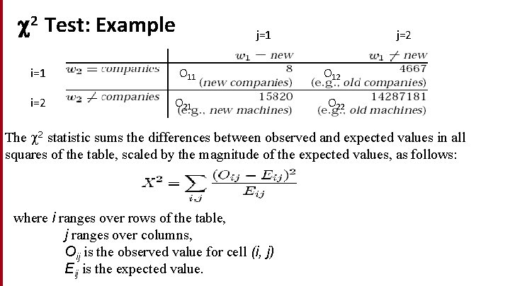
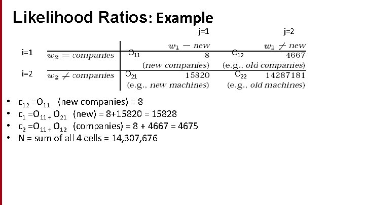
2 Test: Example i=1 i=2 j=1 O 11 O 21 j=2 O 12 O 22 The 2 statistic sums the differences between observed and expected values in all squares of the table, scaled by the magnitude of the expected values, as follows: where i ranges over rows of the table, j ranges over columns, Oij is the observed value for cell (i, j) Eij is the expected value.

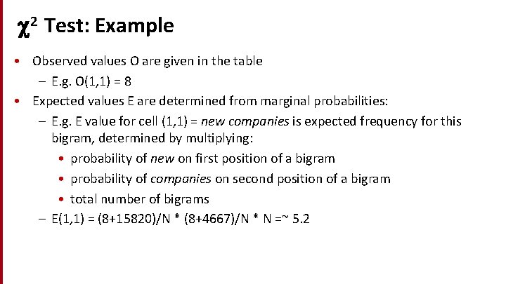
2 Test: Example • Observed values O are given in the table – E. g. O(1, 1) = 8 • Expected values E are determined from marginal probabilities: – E. g. E value for cell (1, 1) = new companies is expected frequency for this bigram, determined by multiplying: • probability of new on first position of a bigram • probability of companies on second position of a bigram • total number of bigrams – E(1, 1) = (8+15820)/N * (8+4667)/N * N =~ 5. 2

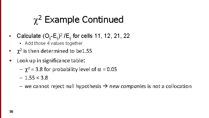
2 Example Continued • Calculate (Oij-Eij)2 /Eij for cells 11, 12, 21, 22 • Add those 4 values together • 2 is then determined to be 1. 55 • Look up in significance table: – 2 = 3. 8 for probability level of = 0. 05 – 1. 55 < 3. 8 – we cannot reject null hypothesis new companies is not a collocation 36

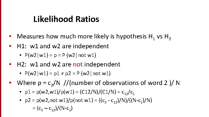
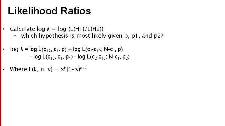
Likelihood Ratios • Measures how much more likely is hypothesis H 1 vs H 2 • H 1: w 1 and w 2 are independent • P(w 2|w 1) = p = P (w 2|not w 1) • H 2: w 1 and w 2 are not independent • P(w 2|w 1) = p 1 ≠ p 2 = P (w 2|not w 1) • Where p = c 2/N //(number of observations of word 2 )/ N • p 1 = p(w 2, w 1)/p(w 1) = (C 12/N)/(C 1/N) = c 12/c 1 • p 2 = p(w 2, not w 1)/p(not w 1) = ((c 2 - c 12)/N)/((N-c 1)/N) = (c 2 – c 12)/(N-c 1)

Likelihood Ratios • Calculate log λ = log (L(H 1)/L(H 2)) • which hypothesis is most likely given p, p 1, and p 2? • log λ = log L(c 12, c 1, p) + log L(c 2 -c 12; N-c 1, p) - log L(c 12, c 1, p 1) - log L(c 2 -c 12; N-c 1, p 2) • Where L(k, n, x) = xk(1 -x)n-k

Likelihood Ratios: Example j=1 i=2 • • O 11 O 21 c 12 =O 11 (new companies) = 8 c 1 =O 11 + O 21 (new) = 8+15820 = 15828 c 2 =O 11 + O 12 (companies) = 8 + 4667 = 4675 N = sum of all 4 cells = 14, 307, 676 j=2 O 12 O 22

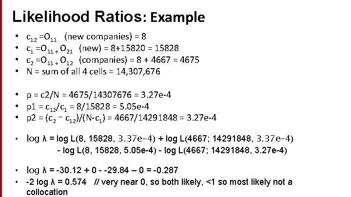
Likelihood Ratios: Example • • c 12 =O 11 (new companies) = 8 c 1 =O 11 + O 21 (new) = 8+15820 = 15828 c 2 =O 11 + O 12 (companies) = 8 + 4667 = 4675 N = sum of all 4 cells = 14, 307, 676 • p = c 2/N = 4675/14307676 = 3. 27 e-4 • p 1 = c 12/c 1 = 8/15828 = 5. 05 e-4 • p 2 = (c 2 – c 12)/(N-c 1) = 4667/14291848 = 3. 27 e-4 • log λ = log L(8, 15828, 3. 37 e-4) + log L(4667; 14291848, 3. 37 e-4) - log L(8, 15828, 5. 05 e-4) - log L(4667; 14291848, 3. 27 e-4) • log λ = -30. 12 + 0 - -29. 84 – 0 = -0. 287 • -2 log λ = 0. 574 // very near 0, so both likely, <1 so most likely not a collocation

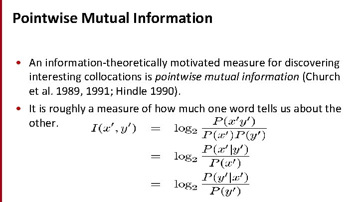
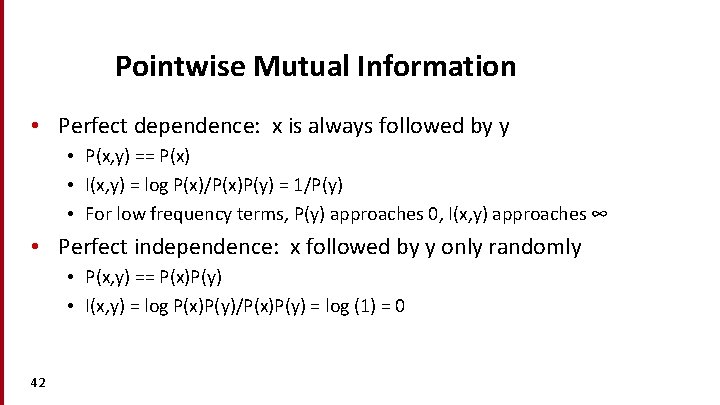
Pointwise Mutual Information • An information-theoretically motivated measure for discovering interesting collocations is pointwise mutual information (Church et al. 1989, 1991; Hindle 1990). • It is roughly a measure of how much one word tells us about the other.

Pointwise Mutual Information • Perfect dependence: x is always followed by y • P(x, y) == P(x) • I(x, y) = log P(x)/P(x)P(y) = 1/P(y) • For low frequency terms, P(y) approaches 0, I(x, y) approaches ∞ • Perfect independence: x followed by y only randomly • P(x, y) == P(x)P(y) • I(x, y) = log P(x)P(y)/P(x)P(y) = log (1) = 0 42

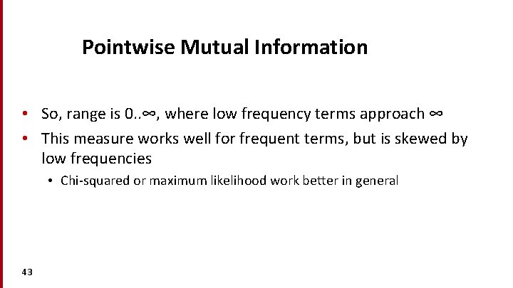
Pointwise Mutual Information • So, range is 0. . ∞, where low frequency terms approach ∞ • This measure works well for frequent terms, but is skewed by low frequencies • Chi-squared or maximum likelihood work better in general 43

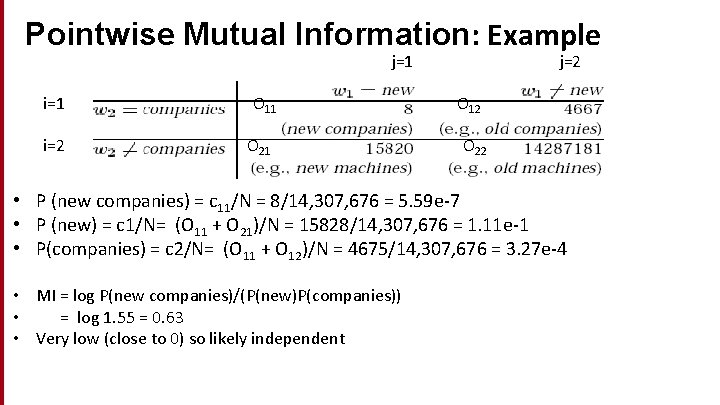
Pointwise Mutual Information: Example j=1 i=2 O 11 O 21 j=2 O 12 O 22 • P (new companies) = c 11/N = 8/14, 307, 676 = 5. 59 e-7 • P (new) = c 1/N= (O 11 + O 21)/N = 15828/14, 307, 676 = 1. 11 e-1 • P(companies) = c 2/N= (O 11 + O 12)/N = 4675/14, 307, 676 = 3. 27 e-4 • MI = log P(new companies)/(P(new)P(companies)) • = log 1. 55 = 0. 63 • Very low (close to 0) so likely independent