CE 5362 Surface Water Modeling 1 D2 D

2 D Diffusion Hydrodynamic Model 2 D horizontal flow – an extension of St.

2 D Diffusion Hydrodynamic Model Sketch of a computational cell x, y directions shown,

2 D Diffusion Hydrodynamic Model Apply continunity principle Where,

2 D Diffusion Hydrodynamic Model Momentum-x Momentum-y

2 D Diffusion Hydrodynamic Model DHM moniker comes from next few steps, where the

2 D Diffusion Hydrodynamic Model First divide momentum by gh

2 D Diffusion Hydrodynamic Model Rename the leftmost three terms “m” (a function of

2 D Diffusion Hydrodynamic Model Stipulate that the friction slope is well approximated by

2 D Diffusion Hydrodynamic Model Rewrite in terms of momentum equations

2 D Diffusion Hydrodynamic Model Substitute into continunity, and the result is a diffusion

2 D Diffusion Hydrodynamic Model Solving takes a trial-and-error approach (hence a lot of

2 D Diffusion Hydrodynamic Model Grid system is complicated, there are 3 grids A

Slides: 18

Download presentation

CE 5362 Surface Water Modeling 1 D/2 D Hydrodynamic Models

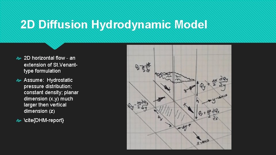
2 D Diffusion Hydrodynamic Model 2 D horizontal flow – an extension of St. Venanttype formulation Assume: Hydrostatic pressure distribution; constant density; planar dimension (x, y) much larger then vertical dimension (z) cite{DHM-report}

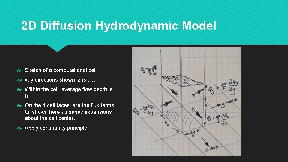
2 D Diffusion Hydrodynamic Model Sketch of a computational cell x, y directions shown, z is up. Within the cell, average flow depth is h On the 4 cell faces, are the flux terms Q, shown here as series expansions about the cell center. Apply continunity principle

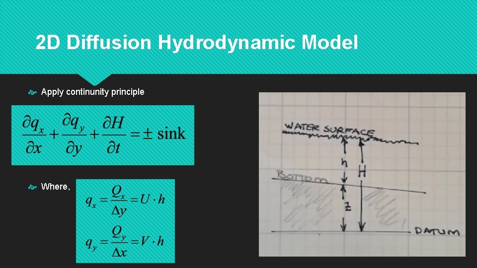
2 D Diffusion Hydrodynamic Model Apply continunity principle Where,

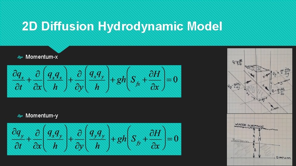
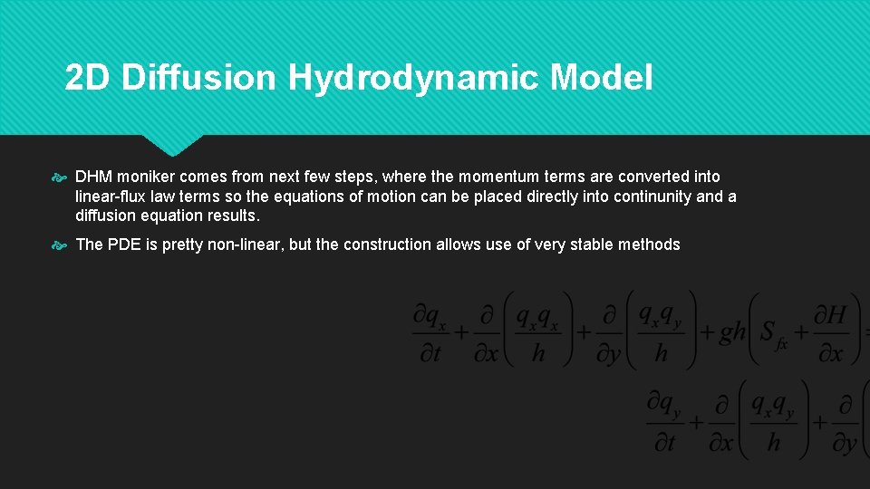
2 D Diffusion Hydrodynamic Model Momentum-x Momentum-y

2 D Diffusion Hydrodynamic Model DHM moniker comes from next few steps, where the momentum terms are converted into linear-flux law terms so the equations of motion can be placed directly into continunity and a diffusion equation results. The PDE is pretty non-linear, but the construction allows use of very stable methods

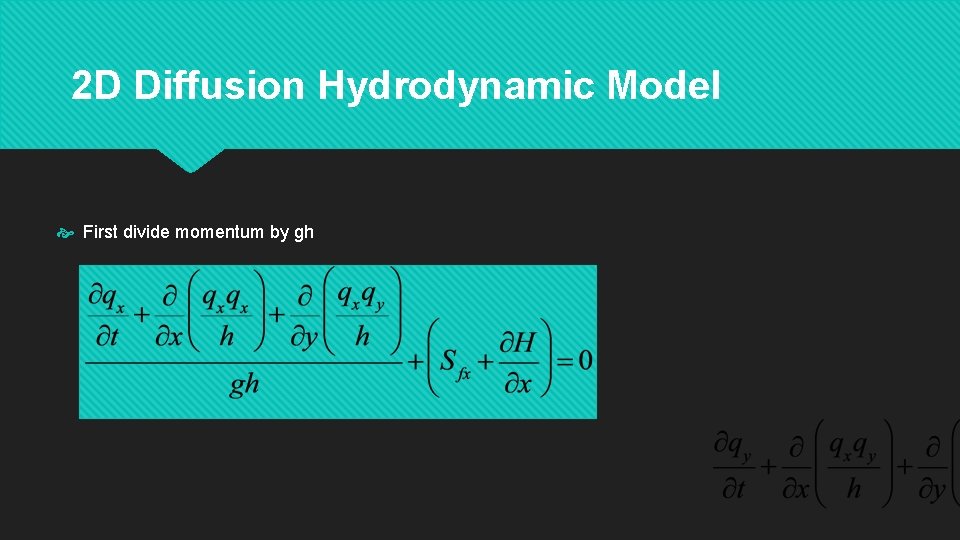
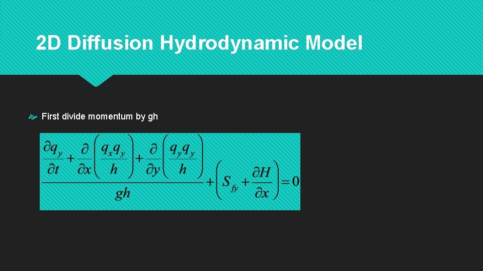
2 D Diffusion Hydrodynamic Model First divide momentum by gh

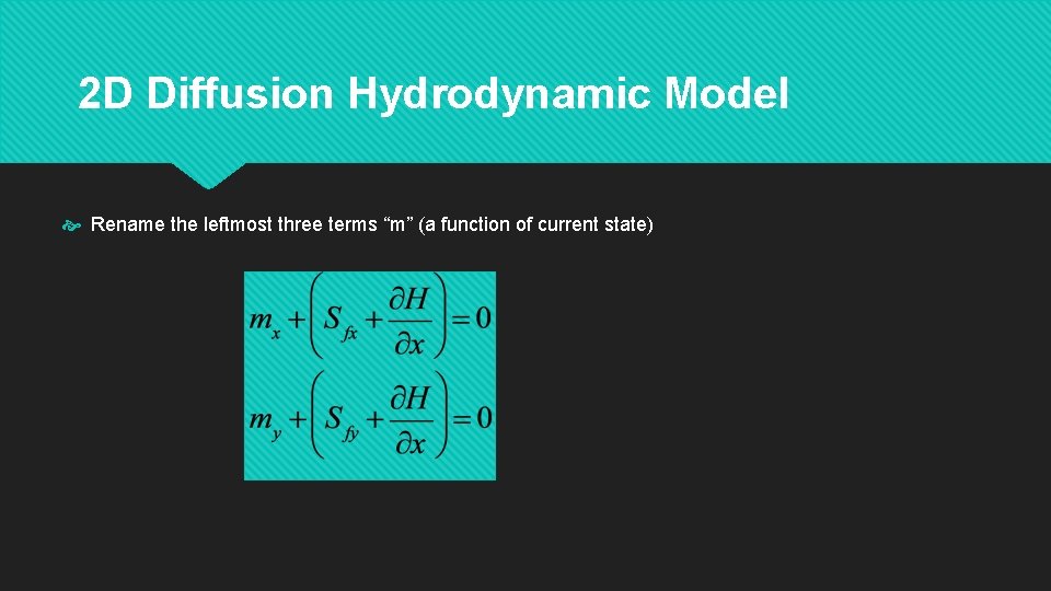
2 D Diffusion Hydrodynamic Model Rename the leftmost three terms “m” (a function of current state)

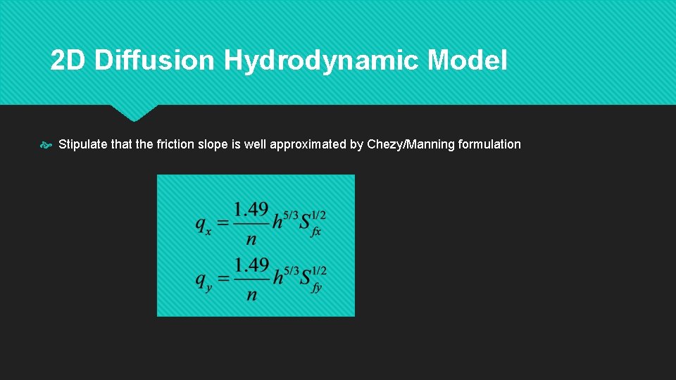
2 D Diffusion Hydrodynamic Model Stipulate that the friction slope is well approximated by Chezy/Manning formulation

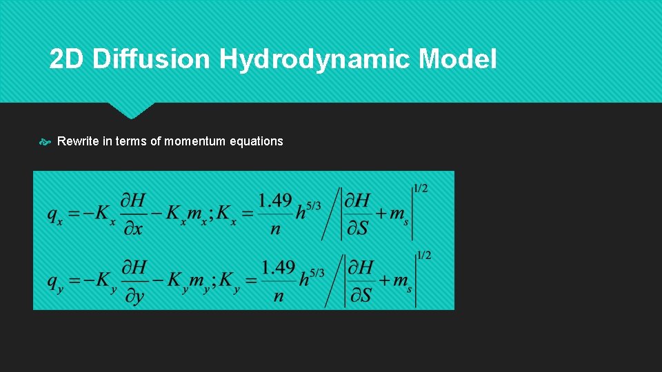
2 D Diffusion Hydrodynamic Model Rewrite in terms of momentum equations

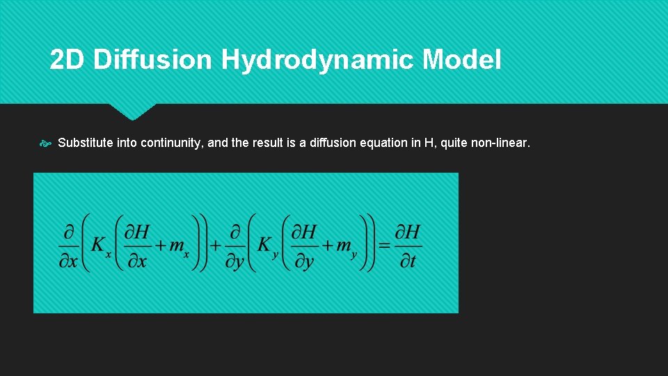
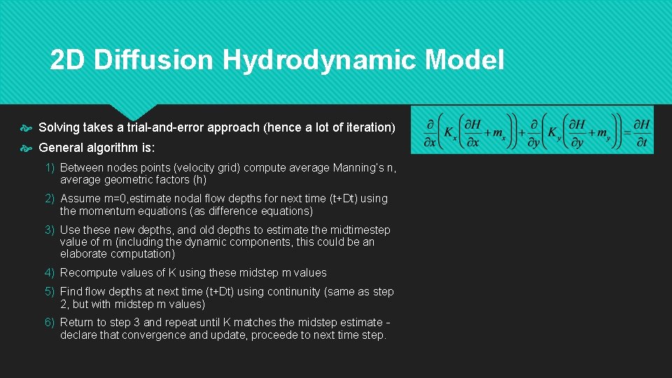
2 D Diffusion Hydrodynamic Model Substitute into continunity, and the result is a diffusion equation in H, quite non-linear.

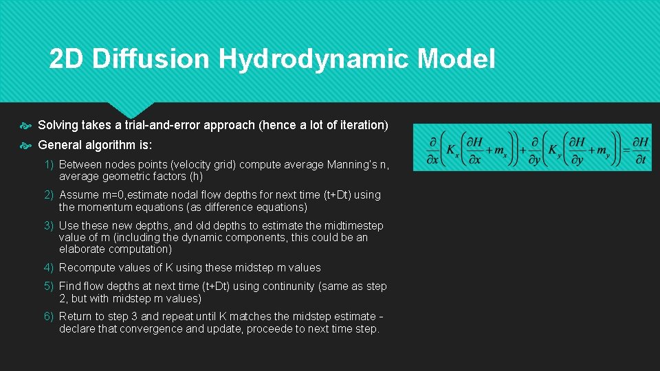
2 D Diffusion Hydrodynamic Model Solving takes a trial-and-error approach (hence a lot of iteration) General algorithm is: 1) Between nodes points (velocity grid) compute average Manning’s n, average geometric factors (h) 2) Assume m=0, estimate nodal flow depths for next time (t+Dt) using the momentum equations (as difference equations) 3) Use these new depths, and old depths to estimate the midtimestep value of m (including the dynamic components, this could be an elaborate computation) 4) Recompute values of K using these midstep m values 5) Find flow depths at next time (t+Dt) using continunity (same as step 2, but with midstep m values) 6) Return to step 3 and repeat until K matches the midstep estimate – declare that convergence and update, proceede to next time step.

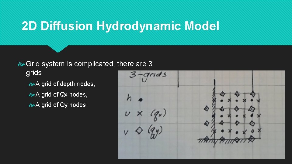
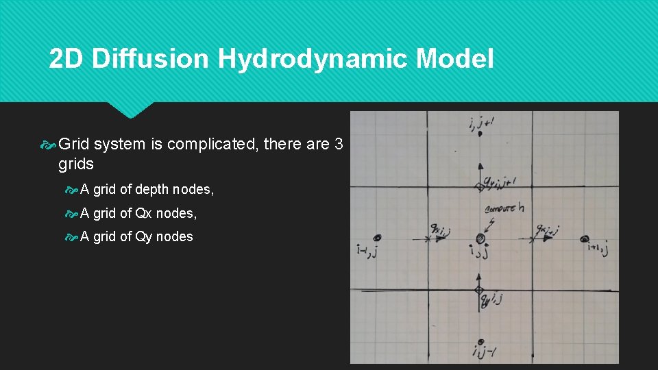
2 D Diffusion Hydrodynamic Model Grid system is complicated, there are 3 grids A grid of depth nodes, A grid of Qx nodes, A grid of Qy nodes

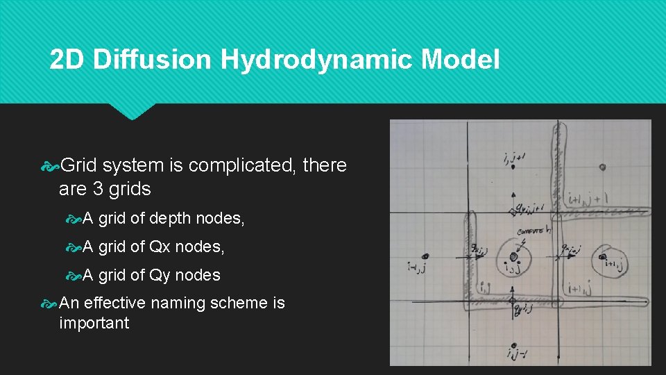
2 D Diffusion Hydrodynamic Model Grid system is complicated, there are 3 grids A grid of depth nodes, A grid of Qx nodes, A grid of Qy nodes An effective naming scheme is important