Calculus Concepts 2e La Torre Kenelly Fetta Harris

Calculus Concepts 2/e La. Torre, Kenelly, Fetta, Harris, and Carpenter Chapter 1 Ingredients of Change: Functions and Linear Models Copyright © by Houghton Mifflin Company, All rights reserved.

Chapter 1 Key Concepts • • • Functions Discrete and Continuous Functions Special Functions Limits of Functions Linear Models Copyright © by Houghton Mifflin Company, All rights reserved.

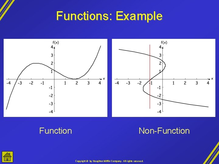
Functions • For every input there is exactly one output. x y 1 2 3 3 3 6 4 6 3 7 7 6 5 8 11 3 8 2 Function Non-Function Copyright © by Houghton Mifflin Company, All rights reserved.

Functions: Example Function Non-Function Copyright © by Houghton Mifflin Company, All rights reserved.

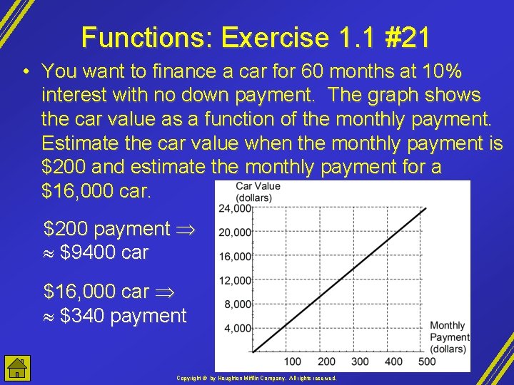
Functions: Exercise 1. 1 #21 • You want to finance a car for 60 months at 10% interest with no down payment. The graph shows the car value as a function of the monthly payment. Estimate the car value when the monthly payment is $200 and estimate the monthly payment for a $16, 000 car. $200 payment $9400 car $16, 000 car $340 payment Copyright © by Houghton Mifflin Company, All rights reserved.

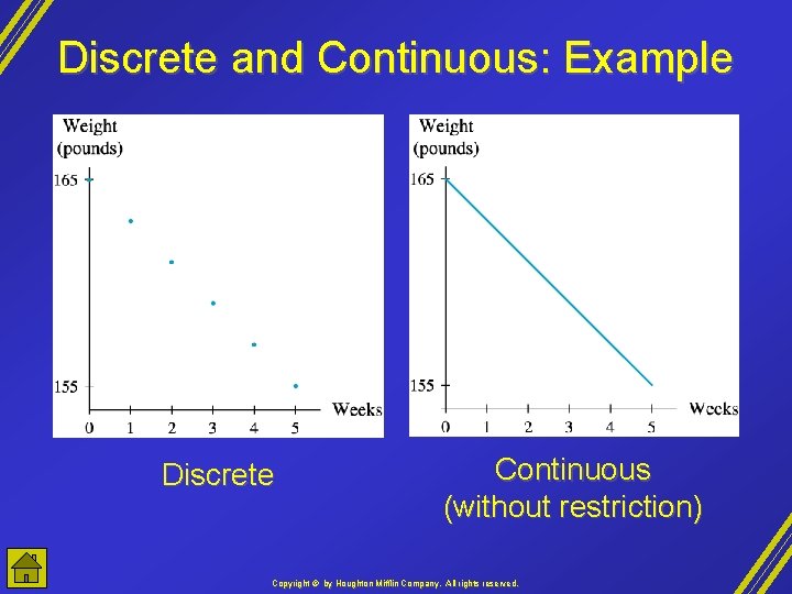
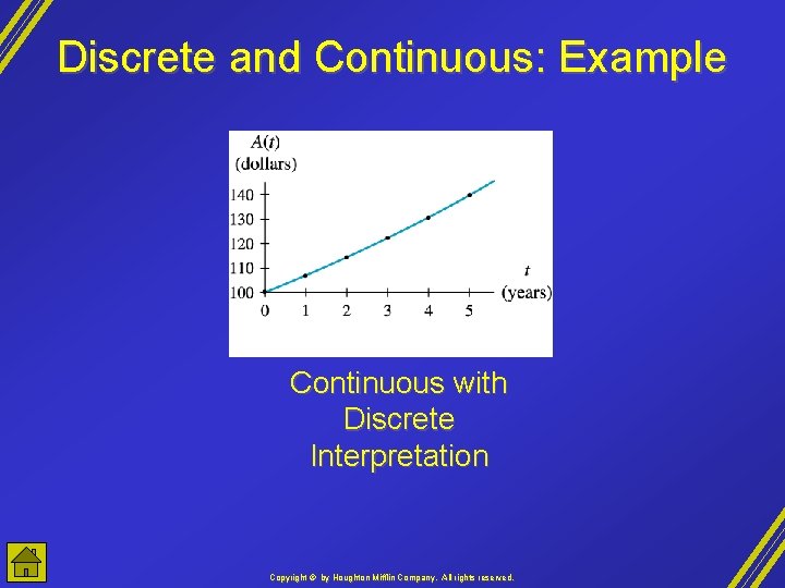
Discrete and Continuous Functions • Discrete - graph is a scatter plot • Continuous - graph doesn’t have any breaks • Continuous with Discrete Interpretation - continuous graph with meaning only at certain points • Continuous without Restriction - continuous graph with meaning at all points Copyright © by Houghton Mifflin Company, All rights reserved.

Discrete and Continuous: Example Discrete Continuous (without restriction) Copyright © by Houghton Mifflin Company, All rights reserved.

Discrete and Continuous: Example Continuous with Discrete Interpretation Copyright © by Houghton Mifflin Company, All rights reserved.

Discrete/Continuous: Exercise 1. 2 #5 • On the basis of data recorded in the spring of each year between 1988 and 1997, the number of students of osteopathic medicine in the U. S. may be modeled as O(t)=0. 027 t 2 - 4. 854 t + 218. 929 thousand students in year 1900 + t. • Is this function discrete, continuous with discrete interpretation or continuous without restriction? • The function is continuous without restriction. Copyright © by Houghton Mifflin Company, All rights reserved.

Special Functions • • • Composite Functions Inverse Functions Piecewise Continuous Functions Copyright © by Houghton Mifflin Company, All rights reserved.

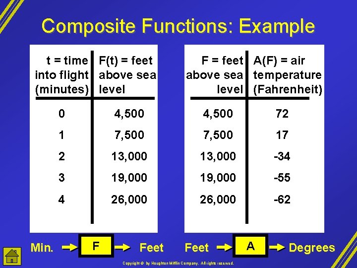
Composite Functions: Example t = time F(t) = feet into flight above sea (minutes) level Min. F = feet A(F) = air above sea temperature level (Fahrenheit) 0 4, 500 72 1 7, 500 17 2 13, 000 -34 3 19, 000 -55 4 26, 000 -62 F Feet Copyright © by Houghton Mifflin Company, All rights reserved. A Degrees

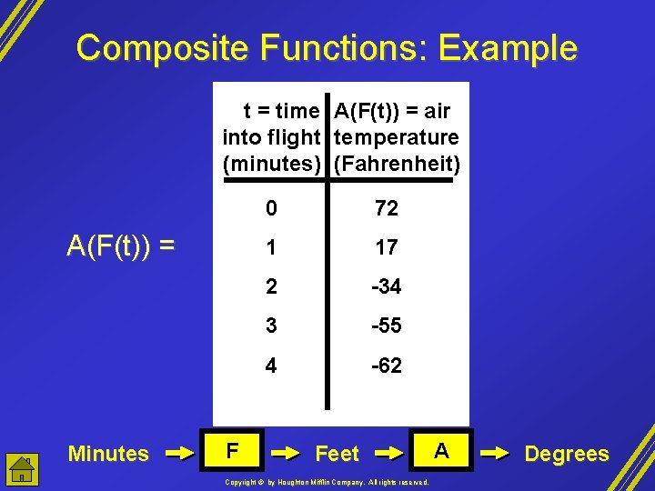
Composite Functions: Example t = time A(F(t)) = air into flight temperature (minutes) (Fahrenheit) A(F(t)) = Minutes F 0 72 1 17 2 -34 3 -55 4 -62 Feet Copyright © by Houghton Mifflin Company, All rights reserved. A Degrees

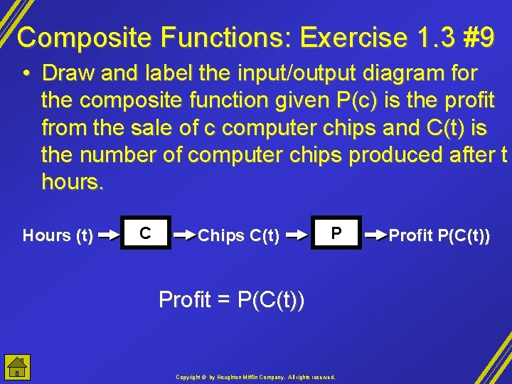
Composite Functions: Exercise 1. 3 #9 • Draw and label the input/output diagram for the composite function given P(c) is the profit from the sale of c computer chips and C(t) is the number of computer chips produced after t hours. Hours (t) C Chips C(t) P Profit = P(C(t)) Copyright © by Houghton Mifflin Company, All rights reserved. Profit P(C(t))

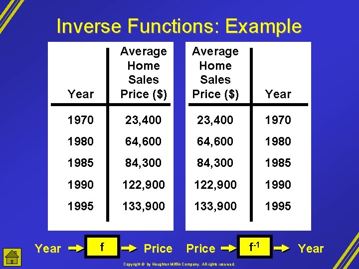
Inverse Functions: Example Year Average Home Sales Price ($) Year 1970 23, 400 1970 1980 64, 600 1985 84, 300 1985 1990 122, 900 1995 133, 900 1995 f Price Copyright © by Houghton Mifflin Company, All rights reserved. f-1 Year

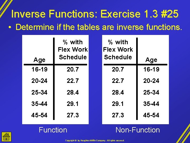
Inverse Functions: Exercise 1. 3 #25 • Determine if the tables are inverse functions. Age % with Flex Work Schedule Age 16 -19 20. 7 16 -19 20 -24 22. 7 20 -24 25 -34 28. 4 25 -34 35 -44 29. 1 35 -44 45 -54 27. 3 45 -54 Function Non-Function Copyright © by Houghton Mifflin Company, All rights reserved.

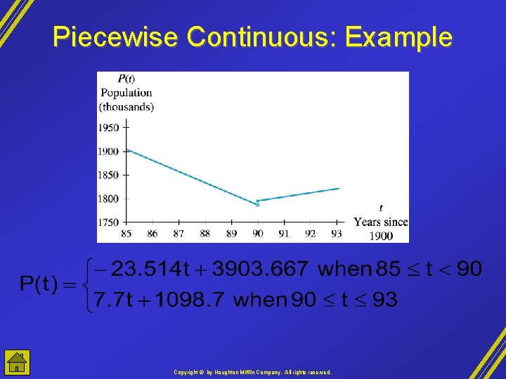
Piecewise Continuous: Example Copyright © by Houghton Mifflin Company, All rights reserved.

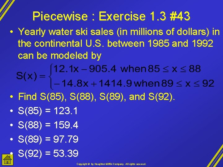
Piecewise : Exercise 1. 3 #43 • Yearly water ski sales (in millions of dollars) in the continental U. S. between 1985 and 1992 can be modeled by • • • Find S(85), S(88), S(89), and S(92). S(85) = 123. 1 S(88) = 159. 4 S(89) = 97. 79 S(92) = 53. 39 Copyright © by Houghton Mifflin Company, All rights reserved.

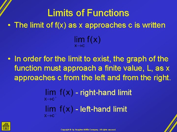
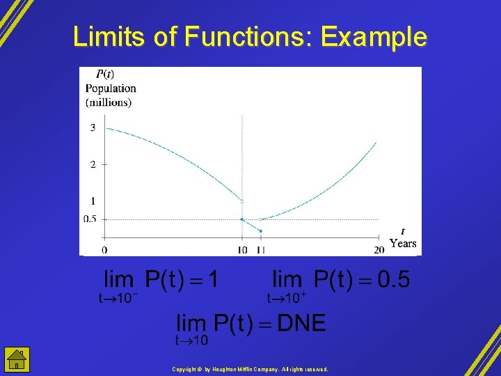
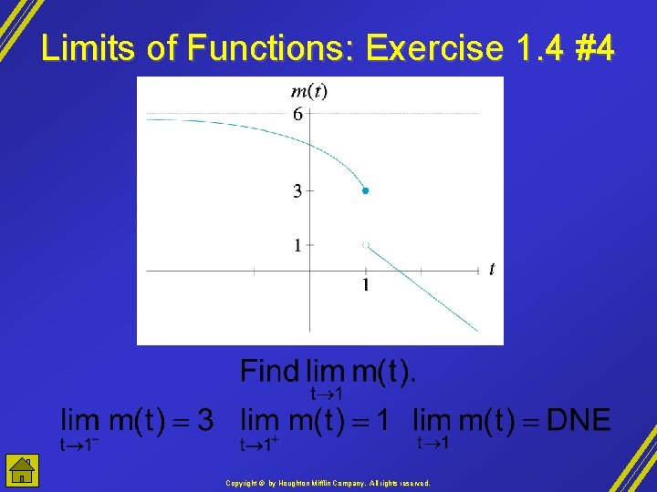
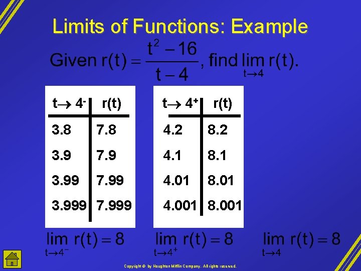
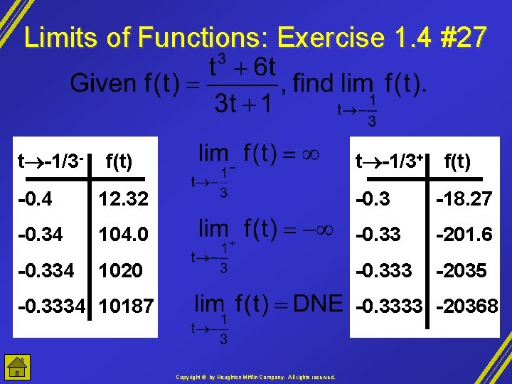
Limits of Functions • The limit of f(x) as x approaches c is written • In order for the limit to exist, the graph of the function must approach a finite value, L, as x approaches c from the left and from the right. - right-hand limit - left-hand limit Copyright © by Houghton Mifflin Company, All rights reserved.

Limits of Functions: Example Copyright © by Houghton Mifflin Company, All rights reserved.

Limits of Functions: Exercise 1. 4 #4 Copyright © by Houghton Mifflin Company, All rights reserved.

Limits of Functions: Example t 4 - r(t) t 4+ r(t) 3. 8 7. 8 4. 2 8. 2 3. 9 7. 9 4. 1 8. 1 3. 99 7. 99 4. 01 8. 01 3. 999 7. 999 4. 001 8. 001 Copyright © by Houghton Mifflin Company, All rights reserved.

Limits of Functions: Exercise 1. 4 #27 t -1/3 - f(t) t -1/3+ f(t) -0. 4 12. 32 -0. 3 -18. 27 -0. 34 104. 0 -0. 33 -201. 6 -0. 334 1020 -0. 333 -2035 -0. 3334 10187 -0. 3333 -20368 Copyright © by Houghton Mifflin Company, All rights reserved.

Linear Models • • • Constant rate of change Equation of form f(x) = ax + b Graph is a line a is the constant rate of change (slope) b is the vertical intercept of the graph of f Copyright © by Houghton Mifflin Company, All rights reserved.

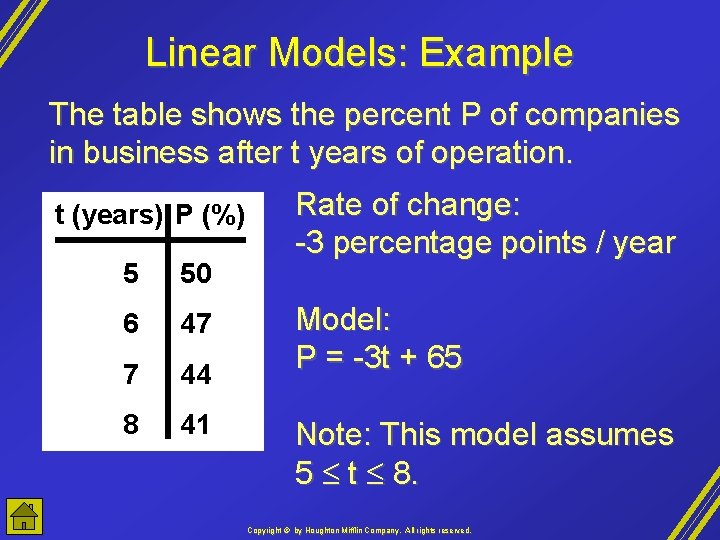
Linear Models: Example The table shows the percent P of companies in business after t years of operation. t (years) P (%) 5 50 6 47 7 44 8 41 Rate of change: -3 percentage points / year Model: P = -3 t + 65 Note: This model assumes 5 t 8. Copyright © by Houghton Mifflin Company, All rights reserved.

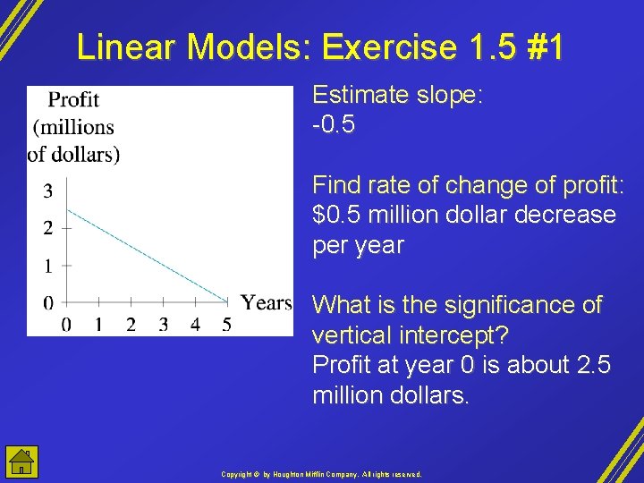
Linear Models: Exercise 1. 5 #1 Estimate slope: -0. 5 Find rate of change of profit: $0. 5 million dollar decrease per year What is the significance of vertical intercept? Profit at year 0 is about 2. 5 million dollars. Copyright © by Houghton Mifflin Company, All rights reserved.