Calculus Concepts 2e La Torre Kenelly Fetta Harris

Calculus Concepts 2/e La. Torre, Kenelly, Fetta, Harris, and Carpenter Chapter 5 Analyzing Change: Applications of Derivatives Copyright © by Houghton Mifflin Company, All rights reserved.

Chapter # Key Concepts • • • Approximating Change Using Tangents Extrema Optimization Without Equations Inflection Points Related Rates Copyright © by Houghton Mifflin Company, All rights reserved.

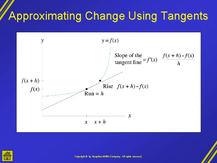
Approximating Change Using Tangents • The change in the tangent line from x to x+h is (slope of tangent line at x) • h • The change in a function from x to x+h can be approximated by the change in the tangent line from x to x+h when h is a small number • That is, f(x+h) - f(x) f '(x) • h • The result of the change in input from x to x+h is f(x+h) f(x) + f '(x) • h Copyright © by Houghton Mifflin Company, All rights reserved.

Approximating Change Using Tangents Copyright © by Houghton Mifflin Company, All rights reserved.

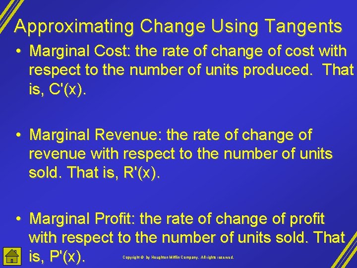
Approximating Change Using Tangents • Marginal Cost: the rate of change of cost with respect to the number of units produced. That is, C'(x). • Marginal Revenue: the rate of change of revenue with respect to the number of units sold. That is, R'(x). • Marginal Profit: the rate of change of profit with respect to the number of units sold. That is, P'(x). Copyright © by Houghton Mifflin Company, All rights reserved.

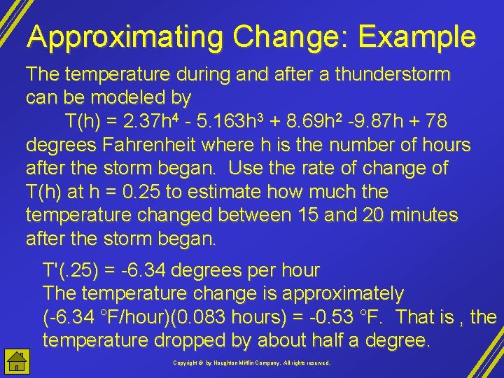
Approximating Change: Example The temperature during and after a thunderstorm can be modeled by T(h) = 2. 37 h 4 - 5. 163 h 3 + 8. 69 h 2 -9. 87 h + 78 degrees Fahrenheit where h is the number of hours after the storm began. Use the rate of change of T(h) at h = 0. 25 to estimate how much the temperature changed between 15 and 20 minutes after the storm began. T'(. 25) = -6. 34 degrees per hour The temperature change is approximately (-6. 34 °F/hour)(0. 083 hours) = -0. 53 °F. That is , the temperature dropped by about half a degree. Copyright © by Houghton Mifflin Company, All rights reserved.

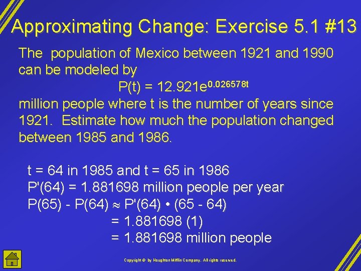
Approximating Change: Exercise 5. 1 #13 The population of Mexico between 1921 and 1990 can be modeled by P(t) = 12. 921 e 0. 026578 t million people where t is the number of years since 1921. Estimate how much the population changed between 1985 and 1986. t = 64 in 1985 and t = 65 in 1986 P'(64) = 1. 881698 million people per year P(65) - P(64) P'(64) • (65 - 64) = 1. 881698 (1) = 1. 881698 million people Copyright © by Houghton Mifflin Company, All rights reserved.

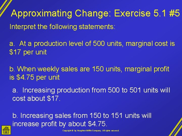
Approximating Change: Exercise 5. 1 #5 Interpret the following statements: a. At a production level of 500 units, marginal cost is $17 per unit b. When weekly sales are 150 units, marginal profit is $4. 75 per unit a. Increasing production from 500 to 501 units will cost about $17. b. Increasing sales from 150 to 151 units will increase profit by about $4. 75. Copyright © by Houghton Mifflin Company, All rights reserved.

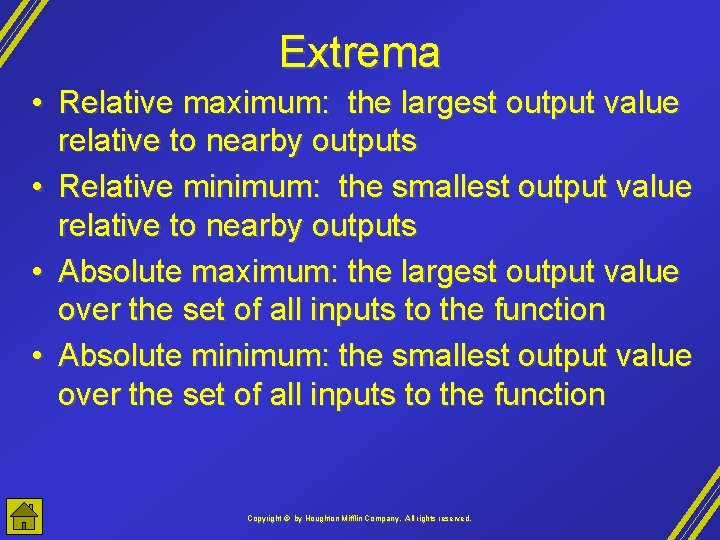
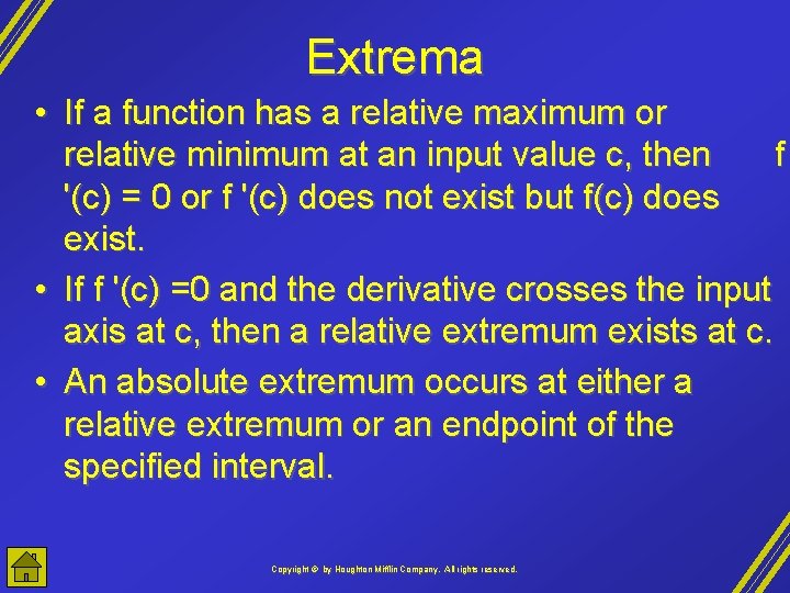
Extrema • Relative maximum: the largest output value relative to nearby outputs • Relative minimum: the smallest output value relative to nearby outputs • Absolute maximum: the largest output value over the set of all inputs to the function • Absolute minimum: the smallest output value over the set of all inputs to the function Copyright © by Houghton Mifflin Company, All rights reserved.

Extrema • If a function has a relative maximum or relative minimum at an input value c, then f '(c) = 0 or f '(c) does not exist but f(c) does exist. • If f '(c) =0 and the derivative crosses the input axis at c, then a relative extremum exists at c. • An absolute extremum occurs at either a relative extremum or an endpoint of the specified interval. Copyright © by Houghton Mifflin Company, All rights reserved.

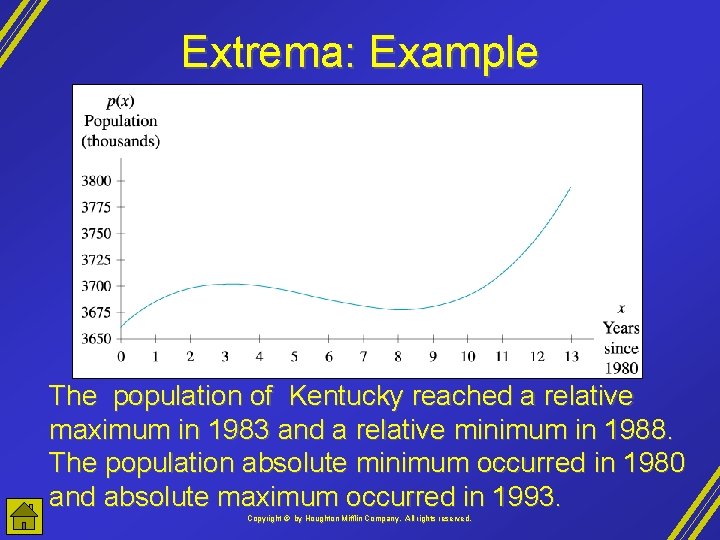
Extrema: Example The population of Kentucky reached a relative maximum in 1983 and a relative minimum in 1988. The population absolute minimum occurred in 1980 and absolute maximum occurred in 1993. Copyright © by Houghton Mifflin Company, All rights reserved.

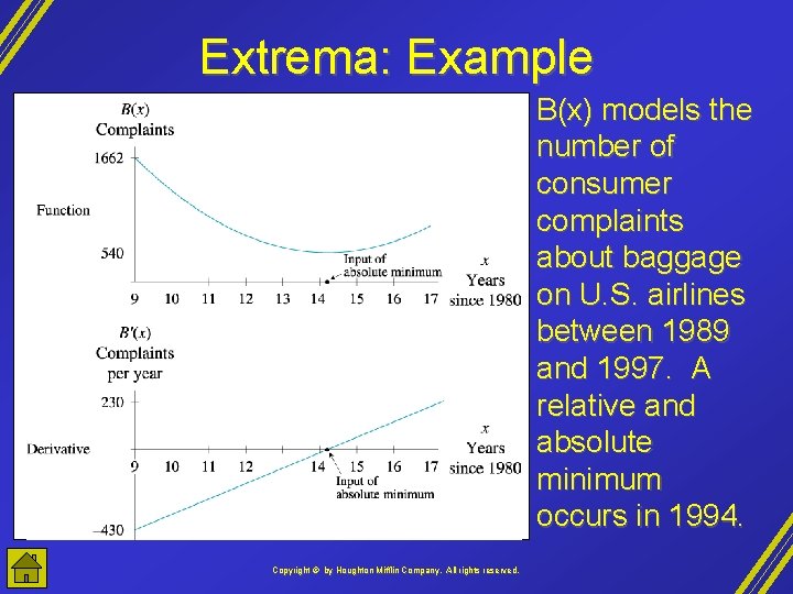
Extrema: Example B(x) models the number of consumer complaints about baggage on U. S. airlines between 1989 and 1997. A relative and absolute minimum occurs in 1994. Copyright © by Houghton Mifflin Company, All rights reserved.

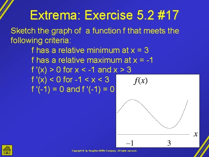
Extrema: Exercise 5. 2 #17 Sketch the graph of a function f that meets the following criteria: f has a relative minimum at x = 3 f has a relative maximum at x = -1 f '(x) > 0 for x < -1 and x > 3 f '(x) < 0 for -1 < x < 3 f '(-1) = 0 and f '(-1) = 0 Copyright © by Houghton Mifflin Company, All rights reserved.

Optimization Without Equations 1 Identify the quantity to be maximized (output) or minimized and the quantity on which the output depends (the input). 2 Sketch and label a picture, if applicable. 3 Build a model for the quantity to be optimized. 4 Rewrite the model equation in terms of only one input variable, if necessary. 5 Identify the input interval. 6 Apply optimization techniques to the equation. 7 Answer the question posed in the problem. Copyright © by Houghton Mifflin Company, All rights reserved.

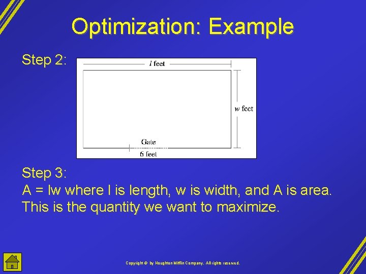
Optimization: Example A rancher removed 200 feet of wire fencing from a field on his ranch. He wishes to reuse the fencing to create a rectangular corral into which he will build a 6 -foot wide wooden gate. What dimensions will result in a corral with the greatest possible area? Step 1: output variable: area of rectangular corral input variables: length and width of corral Copyright © by Houghton Mifflin Company, All rights reserved.

Optimization: Example Step 2: Step 3: A = lw where l is length, w is width, and A is area. This is the quantity we want to maximize. Copyright © by Houghton Mifflin Company, All rights reserved.

Optimization: Example Step 4: The equation is Step 3 has two variables so we need to find a second equation that relates the length and width. 2 w + 2 l - 6 = 200 l = 103 - w So A = lw = (103 - w)w = 103 w - w 2 square feet Step 5: If the corral length is 0 feet, the width is 100 feet. If the corral length is 100 feet, the width is 0 feet. So 0 < w < 100. Copyright © by Houghton Mifflin Company, All rights reserved.

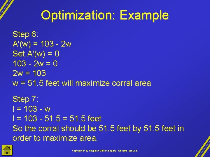
Optimization: Example Step 6: A'(w) = 103 - 2 w Set A'(w) = 0 103 - 2 w = 0 2 w = 103 w = 51. 5 feet will maximize corral area Step 7: l = 103 - w l = 103 - 51. 5 = 51. 5 feet So the corral should be 51. 5 feet by 51. 5 feet in order to maximize area. Copyright © by Houghton Mifflin Company, All rights reserved.

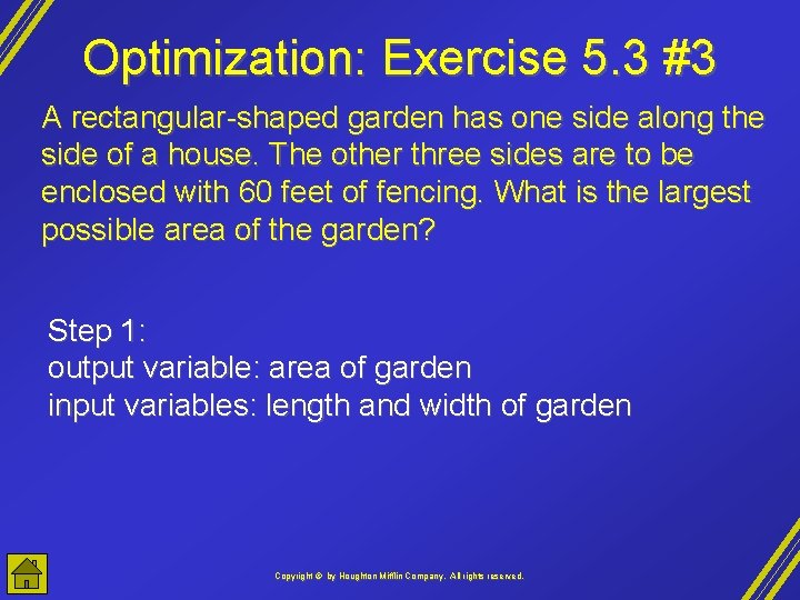
Optimization: Exercise 5. 3 #3 A rectangular-shaped garden has one side along the side of a house. The other three sides are to be enclosed with 60 feet of fencing. What is the largest possible area of the garden? Step 1: output variable: area of garden input variables: length and width of garden Copyright © by Houghton Mifflin Company, All rights reserved.

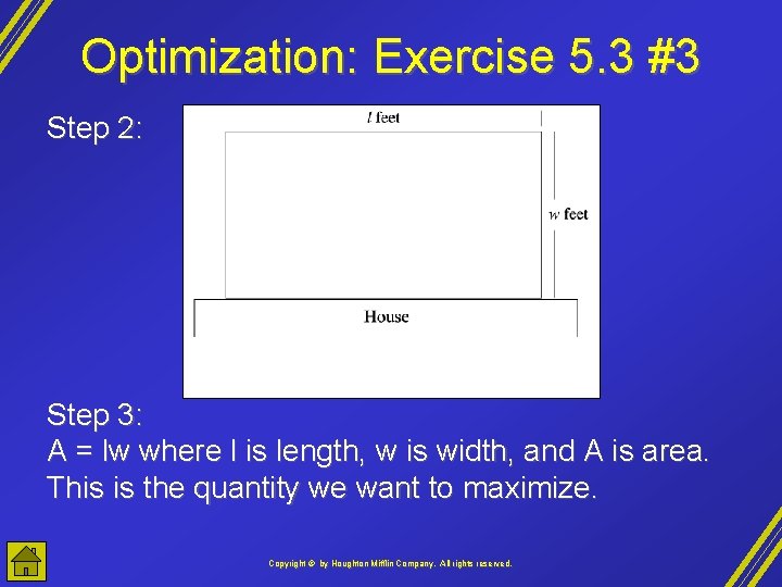
Optimization: Exercise 5. 3 #3 Step 2: Step 3: A = lw where l is length, w is width, and A is area. This is the quantity we want to maximize. Copyright © by Houghton Mifflin Company, All rights reserved.

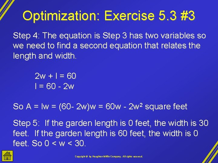
Optimization: Exercise 5. 3 #3 Step 4: The equation is Step 3 has two variables so we need to find a second equation that relates the length and width. 2 w + l = 60 - 2 w So A = lw = (60 - 2 w)w = 60 w - 2 w 2 square feet Step 5: If the garden length is 0 feet, the width is 30 feet. If the garden length is 60 feet, the width is 0 feet. So 0 < w < 30. Copyright © by Houghton Mifflin Company, All rights reserved.

Optimization: Exercise 5. 3 #3 Step 6: A'(w) = 60 - 4 w Set A'(w) = 0 60 - 4 w = 0 4 w = 60 w = 15 feet will maximize garden area Step 7: l = 60 - 2 w l = 60 - 2(15) = 30 feet The garden should be 15 feet by 30 feet in order to maximize area. The long side is against the house. Copyright © by Houghton Mifflin Company, All rights reserved.

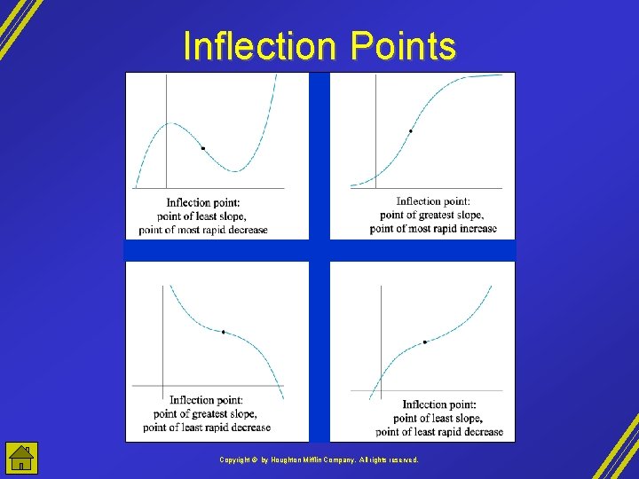
Inflection Points • inflection point: a point where the graph changes concavity • If c is an inflection point of a function f then f ''(c) = 0 or f ''(c) is undefined • If the second derivative graph crosses the horizontal axis, then an inflection point of the function graph occurs at that input value. Copyright © by Houghton Mifflin Company, All rights reserved.

Inflection Points Copyright © by Houghton Mifflin Company, All rights reserved.

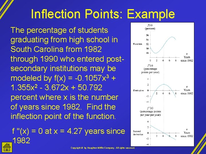
Inflection Points: Example The percentage of students graduating from high school in South Carolina from 1982 through 1990 who entered postsecondary institutions may be modeled by f(x) = -0. 1057 x 3 + 1. 355 x 2 - 3. 672 x + 50. 792 percent where x is the number of years since 1982. Find the inflection point of the function. f ''(x) = 0 at x = 4. 27 years since 1982 Copyright © by Houghton Mifflin Company, All rights reserved.

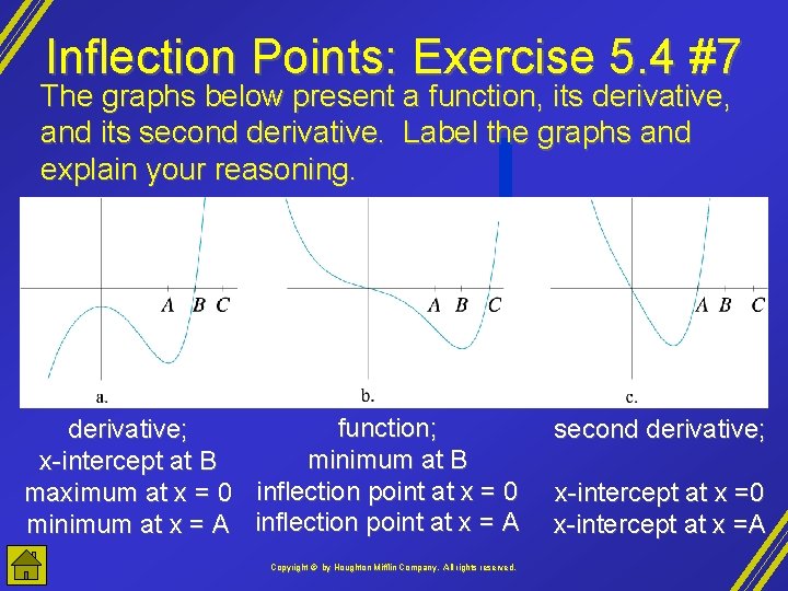
Inflection Points: Exercise 5. 4 #7 The graphs below present a function, its derivative, and its second derivative. Label the graphs and explain your reasoning. function; derivative; minimum at B x-intercept at B maximum at x = 0 inflection point at x = 0 minimum at x = A inflection point at x = A Copyright © by Houghton Mifflin Company, All rights reserved. second derivative; x-intercept at x =0 x-intercept at x =A

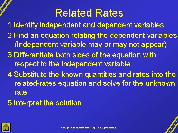
Related Rates 1 Identify independent and dependent variables 2 Find an equation relating the dependent variables. (Independent variable may or may not appear) 3 Differentiate both sides of the equation with respect to the independent variable 4 Substitute the known quantities and rates into the related-rates equation and solve for the unknown rate 5 Interpret the solution Copyright © by Houghton Mifflin Company, All rights reserved.

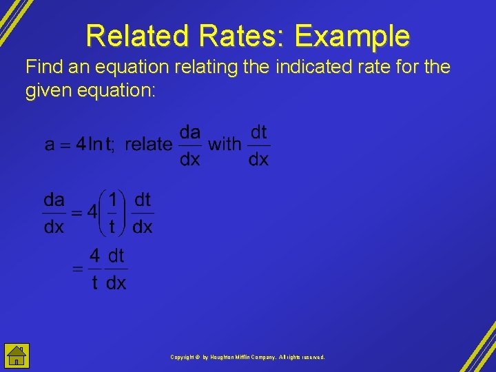
Related Rates: Example Find an equation relating the indicated rate for the given equation: Copyright © by Houghton Mifflin Company, All rights reserved.

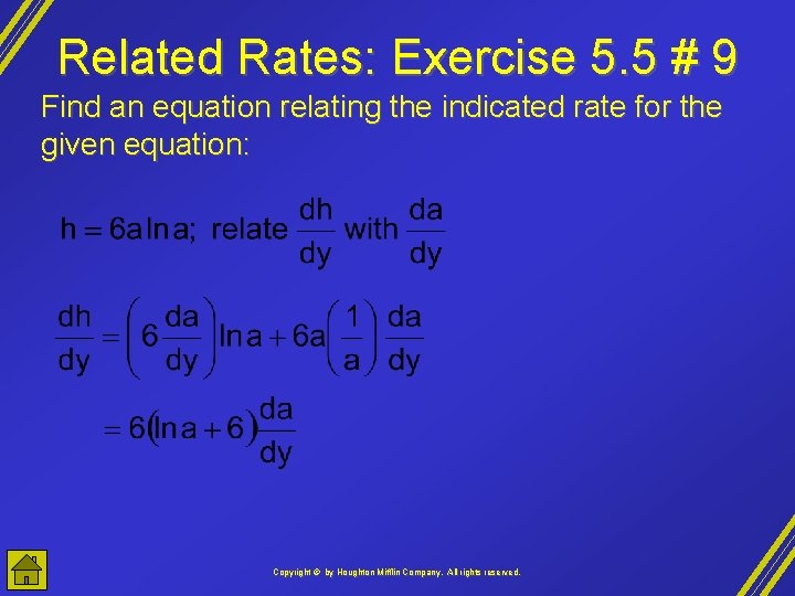
Related Rates: Exercise 5. 5 # 9 Find an equation relating the indicated rate for the given equation: Copyright © by Houghton Mifflin Company, All rights reserved.