Calculus Concepts 2e La Torre Kenelly Fetta Harris






- Slides: 30

Calculus Concepts 2/e La. Torre, Kenelly, Fetta, Harris, and Carpenter Chapter 6 Accumulating Change: Limits of Sums and the Definite Integral Copyright © by Houghton Mifflin Company, All rights reserved.

Chapter 6 Key Concepts • • Results of Change Approximating Area with Rectangles Limits of Sums of Rectangle Areas Introduction to Accumulation Functions Fundamental Theorem and Antiderivatives Definite Integrals Improper Integrals Copyright © by Houghton Mifflin Company, All rights reserved.

Results of Change • The accumulated change in a quantity is represented as the area or signed area of a region between the rate-of-change function for that quantity and the horizontal axis provided the function does not cross the horizontal axis. Copyright © by Houghton Mifflin Company, All rights reserved.

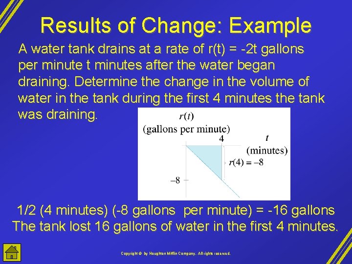
Results of Change: Example A water tank drains at a rate of r(t) = -2 t gallons per minute t minutes after the water began draining. Determine the change in the volume of water in the tank during the first 4 minutes the tank was draining. 1/2 (4 minutes) (-8 gallons per minute) = -16 gallons The tank lost 16 gallons of water in the first 4 minutes. Copyright © by Houghton Mifflin Company, All rights reserved.

Results of Change: Exercise 6. 1 #15 The rate of change of the population of North Dakota from 1970 through 1990 is modeled on the graph below. Find the area between the graph of p and the horizontal axis from 0 to 15 and interpret. (3870 people per year)(15 years) = 58, 050 people From 1970 to 1985, the population of North Dakota increased by 58, 050 people. Copyright © by Houghton Mifflin Company, All rights reserved.

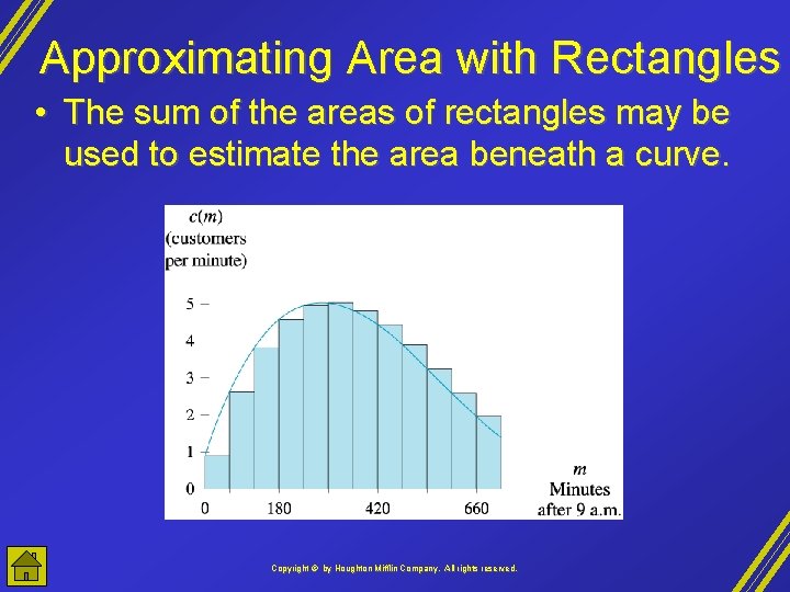
Approximating Area with Rectangles • The sum of the areas of rectangles may be used to estimate the area beneath a curve. Copyright © by Houghton Mifflin Company, All rights reserved.

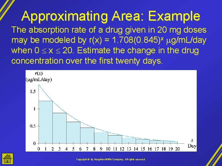
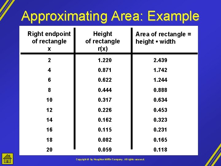
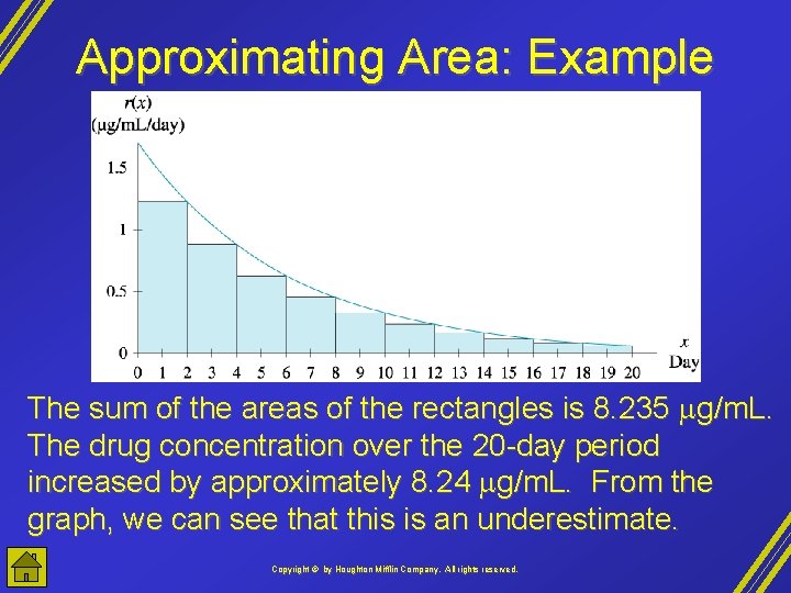
Approximating Area: Example The absorption rate of a drug given in 20 mg doses may be modeled by r(x) = 1. 708(0. 845)x g/m. L/day when 0 x 20. Estimate the change in the drug concentration over the first twenty days. Copyright © by Houghton Mifflin Company, All rights reserved.

Approximating Area: Example Right endpoint of rectangle x Height of rectangle r(x) Area of rectangle = height • width 2 1. 220 2. 439 4 0. 871 1. 742 6 0. 622 1. 244 8 0. 444 0. 888 10 0. 317 0. 634 12 0. 226 0. 453 14 0. 162 0. 323 16 0. 115 0. 231 18 0. 082 0. 165 20 0. 059 0. 118 Copyright © by Houghton Mifflin Company, All rights reserved.

Approximating Area: Example The sum of the areas of the rectangles is 8. 235 g/m. L. The drug concentration over the 20 -day period increased by approximately 8. 24 g/m. L. From the graph, we can see that this is an underestimate. Copyright © by Houghton Mifflin Company, All rights reserved.

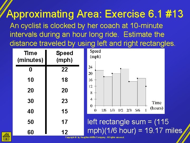
Approximating Area: Exercise 6. 1 #13 An cyclist is clocked by her coach at 10 -minute intervals during an hour long ride. Estimate the distance traveled by using left and right rectangles. Time (minutes) Speed (mph) 0 22 10 18 20 20 30 23 40 15 50 17 60 12 left rectangle sum = (115 mph)(1/6 hour) = 19. 17 miles Copyright © by Houghton Mifflin Company, All rights reserved.

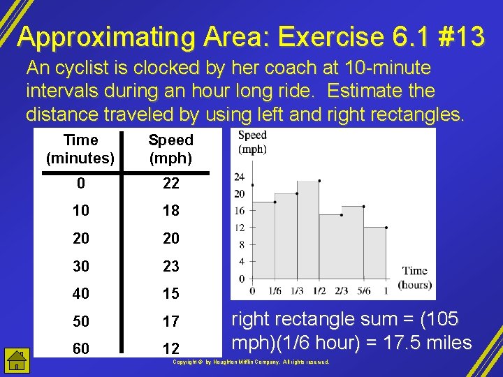
Approximating Area: Exercise 6. 1 #13 An cyclist is clocked by her coach at 10 -minute intervals during an hour long ride. Estimate the distance traveled by using left and right rectangles. Time (minutes) Speed (mph) 0 22 10 18 20 20 30 23 40 15 50 17 60 12 right rectangle sum = (105 mph)(1/6 hour) = 17. 5 miles Copyright © by Houghton Mifflin Company, All rights reserved.

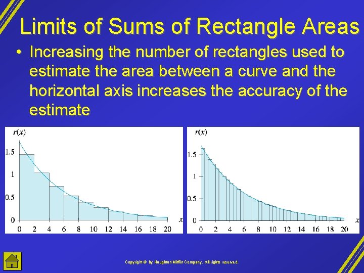
Limits of Sums of Rectangle Areas • Increasing the number of rectangles used to estimate the area between a curve and the horizontal axis increases the accuracy of the estimate Copyright © by Houghton Mifflin Company, All rights reserved.

Limits of Sums of Rectangle Areas • Let f be a continuous or piecewise continuous non-negative function from a to b. The area of the region between the graph of f and the xaxis from a to b is given by the limit where x 1, x 2, . . . , xn are the midpoints of n subintervals of length x = (b-a)/n between a and b. is called the definite integral of f from a to b. Copyright © by Houghton Mifflin Company, All rights reserved.

Limits of Sums: Example The flow rates of the Carson River can be modeled by f(x) = 18, 225 x 2 -135, 334. 3 x + 2, 881, 542. 9 ft 3/hr where x is the number of hours after 11: 45 a. m. Wednesday. Use the idea of limit of sums to estimate to the nearest ten thousand cubic feet the amount of water that flowed through the river from 11: 45 a. m. on Wednesday to 7: 45 a. m. on Thursday. We need to find the area between the curve and the x-axis from x = 0 to x = 20. We’ll use midpoint rectangles. Copyright © by Houghton Mifflin Company, All rights reserved.

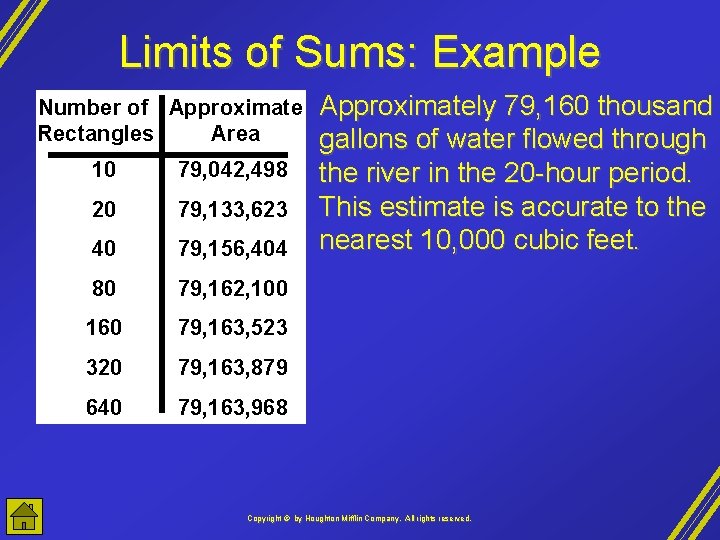
Limits of Sums: Example Number of Approximate Rectangles Area 10 79, 042, 498 20 79, 133, 623 40 79, 156, 404 80 79, 162, 100 160 79, 163, 523 320 79, 163, 879 640 79, 163, 968 Approximately 79, 160 thousand gallons of water flowed through the river in the 20 -hour period. This estimate is accurate to the nearest 10, 000 cubic feet. Copyright © by Houghton Mifflin Company, All rights reserved.

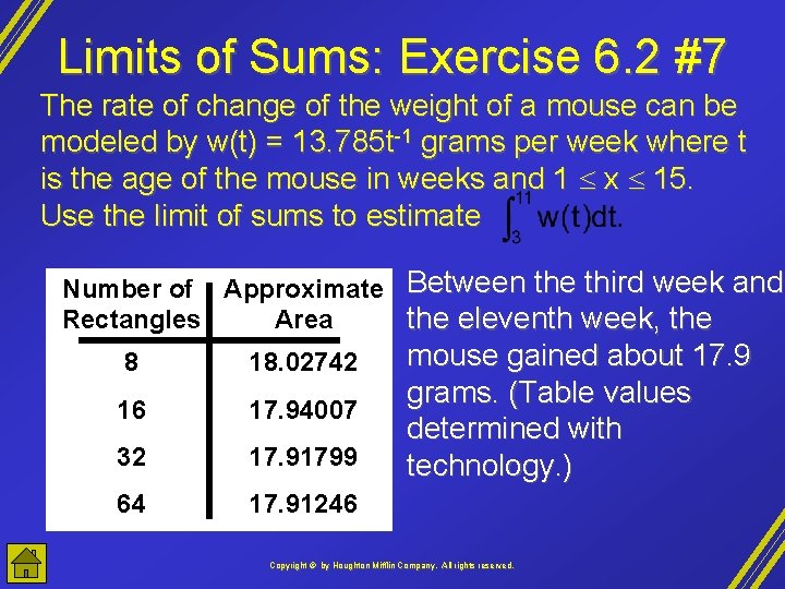
Limits of Sums: Exercise 6. 2 #7 The rate of change of the weight of a mouse can be modeled by w(t) = 13. 785 t-1 grams per week where t is the age of the mouse in weeks and 1 x 15. Use the limit of sums to estimate Number of Approximate Between the third week and Rectangles Area the eleventh week, the 8 18. 02742 16 17. 94007 32 17. 91799 64 17. 91246 mouse gained about 17. 9 grams. (Table values determined with technology. ) Copyright © by Houghton Mifflin Company, All rights reserved.

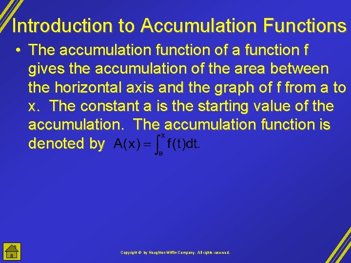
Introduction to Accumulation Functions • The accumulation function of a function f gives the accumulation of the area between the horizontal axis and the graph of f from a to x. The constant a is the starting value of the accumulation. The accumulation function is denoted by Copyright © by Houghton Mifflin Company, All rights reserved.

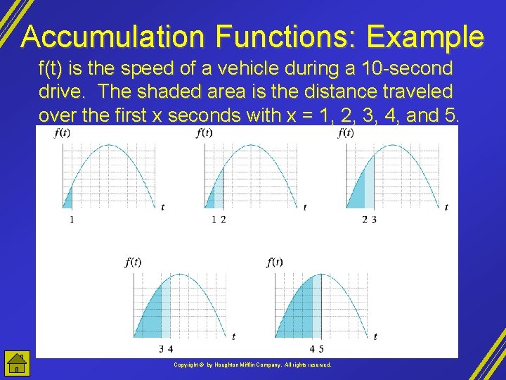
Accumulation Functions: Example f(t) is the speed of a vehicle during a 10 -second drive. The shaded area is the distance traveled over the first x seconds with x = 1, 2, 3, 4, and 5. Copyright © by Houghton Mifflin Company, All rights reserved.

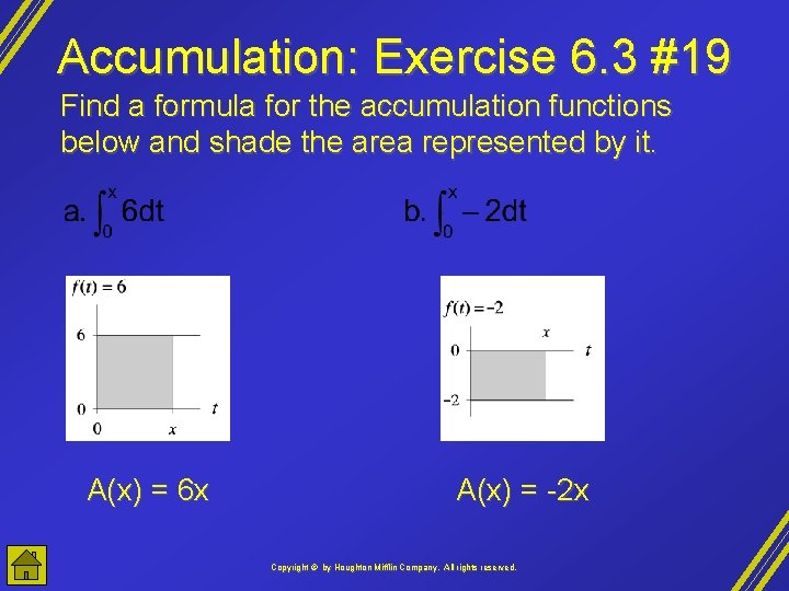
Accumulation: Exercise 6. 3 #19 Find a formula for the accumulation functions below and shade the area represented by it. A(x) = 6 x A(x) = -2 x Copyright © by Houghton Mifflin Company, All rights reserved.

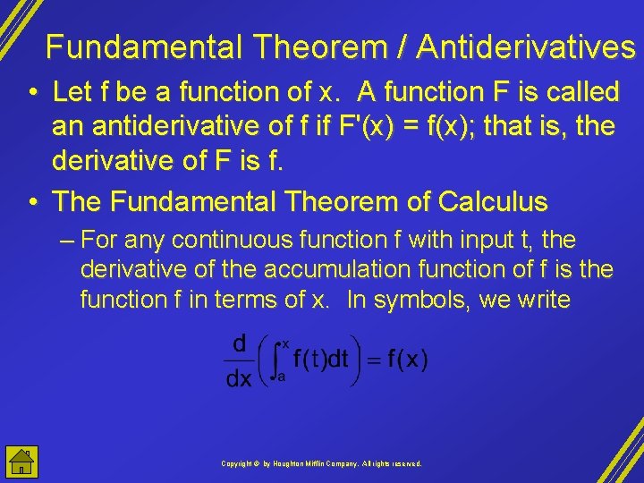
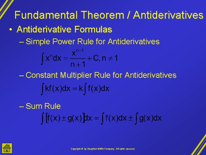
Fundamental Theorem / Antiderivatives • Let f be a function of x. A function F is called an antiderivative of f if F'(x) = f(x); that is, the derivative of F is f. • The Fundamental Theorem of Calculus – For any continuous function f with input t, the derivative of the accumulation function of f is the function f in terms of x. In symbols, we write Copyright © by Houghton Mifflin Company, All rights reserved.

Fundamental Theorem / Antiderivatives • Antiderivative Formulas – Simple Power Rule for Antiderivatives – Constant Multiplier Rule for Antiderivatives – Sum Rule Copyright © by Houghton Mifflin Company, All rights reserved.

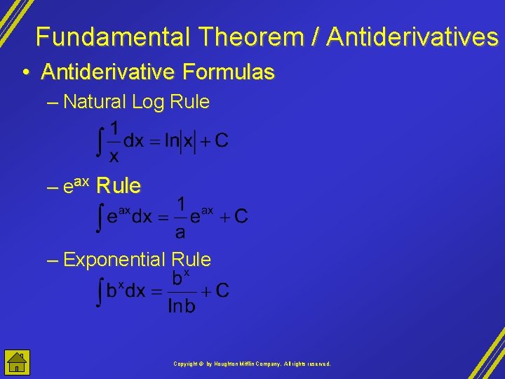
Fundamental Theorem / Antiderivatives • Antiderivative Formulas – Natural Log Rule – eax Rule – Exponential Rule Copyright © by Houghton Mifflin Company, All rights reserved.

Fundamental Thm. / Antiderivatives: Example An African country has an increasing population but a declining birth rate. The rate of change in the number of babies born each year is given by b(t) = 87, 000 - 1600 t births per year t years from the end of this year. The number of babies born this year is 1, 185, 800. Find a function describing the number of births each year t years from now. Copyright © by Houghton Mifflin Company, All rights reserved.

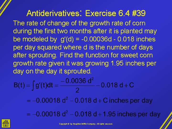
Antiderivatives: Exercise 6. 4 #39 The rate of change of the growth rate of corn during the first two months after it is planted may be modeled by g'(d) = -0. 00036 d - 0. 018 inches per day squared where d is the number of days after sprouting. Find the function for sweet corn growth rate given it was growing 1. 95 inches per day on the day it sprouted. Copyright © by Houghton Mifflin Company, All rights reserved.

Definite Integrals • If f is a continuous function from a to b and F is any antiderivative of f, then • The definite integral from a to b represents the total change in F over the interval a to b Copyright © by Houghton Mifflin Company, All rights reserved.

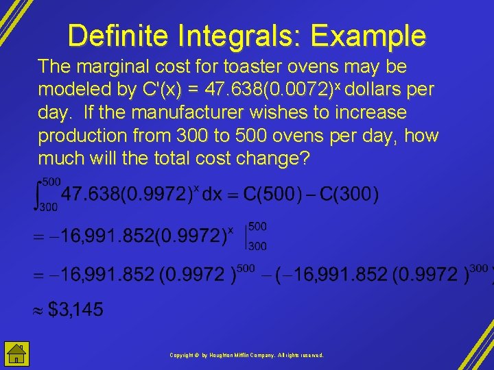
Definite Integrals: Example The marginal cost for toaster ovens may be modeled by C'(x) = 47. 638(0. 0072)x dollars per day. If the manufacturer wishes to increase production from 300 to 500 ovens per day, how much will the total cost change? Copyright © by Houghton Mifflin Company, All rights reserved.

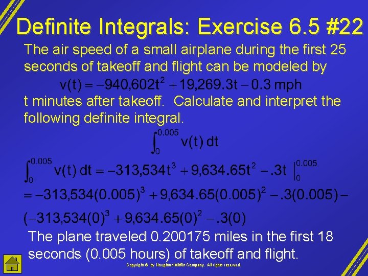
Definite Integrals: Exercise 6. 5 #22 The air speed of a small airplane during the first 25 seconds of takeoff and flight can be modeled by t minutes after takeoff. Calculate and interpret the following definite integral. The plane traveled 0. 200175 miles in the first 18 seconds (0. 005 hours) of takeoff and flight. Copyright © by Houghton Mifflin Company, All rights reserved.

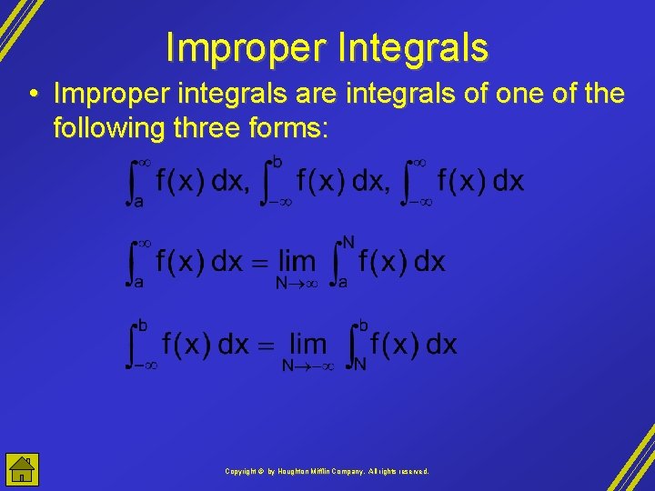
Improper Integrals • Improper integrals are integrals of one of the following three forms: Copyright © by Houghton Mifflin Company, All rights reserved.

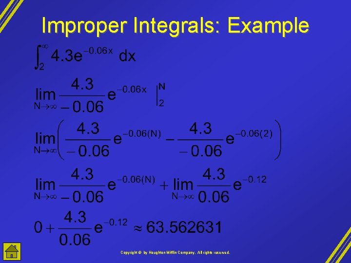
Improper Integrals: Example Copyright © by Houghton Mifflin Company, All rights reserved.

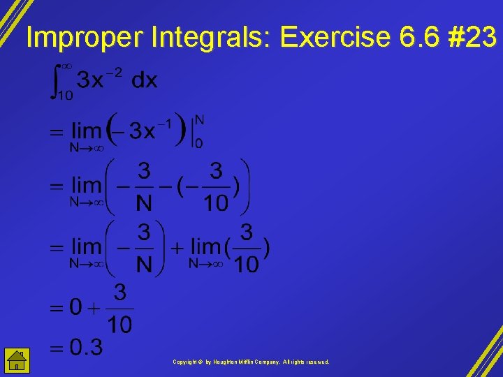
Improper Integrals: Exercise 6. 6 #23 Copyright © by Houghton Mifflin Company, All rights reserved.