Atmospheric Soundings and simpler algorithms Atmospheric absorption spectrum
")
Atmospheric Soundings (and simpler algorithms)

Atmospheric absorption spectrum at 10 km. Zenith angle of observation: 30. Terrestrial concentration 1.
 as")
Fig. 7. 23 Demonstrative atmospheric transmittances (total, H 2 O and O 2) as a function of frequency and wavelength in the microwave region. (From An Introduction to Atmospheric Radiation, 2002, Liou, K. N. p. 415. )
 y = Data: Forward")
Minimum Variance Sol‘n (Few, and independent state variables, little noise) y = Data: Forward Model: x = State Vector Variables: Radiances Radiative Transfer Sfc Temp Ch. 1, 2, & 3 + Sfc wind speed (ocean) Assumption Total Column Water Vapor e. g. Temperature, water vapor & pressure profile Solution: Guess x, iterate until y is close to F(x)

Radiative transfer equation in terms of transmission: In terms of physical height z: The factor weights the Planck function, B(z).

A simple interpretation of the solution Integral emission Surface term 1 T 2 T 3 Ts 3 2

Examples: 1: 2: 3:

Weighting Functions for Limb Sounding Radiative transfer equation: where is the path through the atmosphere.

Advantages of Limb Sounding by Emission • None of the emitted radiation seen by the satellite originates below the tangent height: allows for relatively high vertical resolution. • The surface has no influence on the measured intensities. • Due to the geometry of limb sounding, considerably more emitting gas is encountered along grazing paths than on straight ones increasing the instrument sensitivity to gases of low concentration. • Also, due to paths being high in the atmosphere, effects of pressure broadening are reduced. Disadvantages of Limb Sounding by Emission • Very sensitive to aerosol in the lower stratosphere. • Cannot be used in the troposphere because atmosphere is too optically thick.

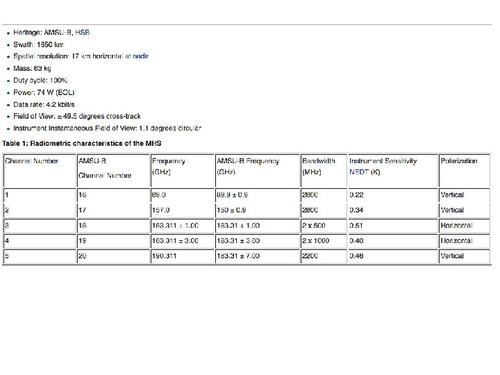
Microwave Systems Imagers Sounders SSMI TMI Wind. Sat AMSR-E AMSR 2 GMI MSU SSMT 2 AMSU MHS ATMS Imagers/Sounders SSMIS

13

Multispectral Imagery in the Optical Spectrum Absorption Bands O 3 CO 2 H 2 O Question: why are there warm spikes located in the deepest parts of the major absorption bands? 14

15

16

An Introduction to Optimal Estimation Theory

The Bible of Optimal Estimation: Rodgers, 2000
 + NOISE OR DATA:")
The Retrieval PROBLEM DATA = FORWARD MODEL ( State ) + NOISE OR DATA: Forward Model: Reflectivities Radiative Transfer Radiances + Radar Backscatter Assumption e. g. Emissivity pressure State Vector Variables: Temperatures Water Vapor Cloud Variables Noise: Instrument Noise Forward Model Error Sub grid-scale processes

We must invert this equation to get x, but how to do this: • When there are different numbers of unknown variables as measured variables? • In the presence of noise? • When F(x) is nonlinear (often highly) ? • When the observations are not independent?
 DATA: TB‘s (m, 1) col vector Forward Model: (m, n)")
Mathematical Setup (linear problem) DATA: TB‘s (m, 1) col vector Forward Model: (m, n) matrix State Vector Variables: Temp Profile (n, 1) col vector

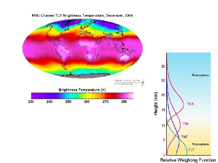
Hypothetical Temperature Retrieval Temperature Profile Temperature Weighting Functions

• If we assume no prior constraint on x, we can write an equation for the cost fucntion c, where Sy is the errror covariance Can now simply minimize c 2 w. r. t. x • The error covariance now takes care of channels with more or less certainty.

Generalized Error Covariance Matrix • Variables: y 1, y 2 , y 3. . . • 1 -sigma errors: 1 , 2 , 3. . . • The correlation between error on y 1 and error on y 2 is c 12 (between – 1 and 1), etc. • Then, the Measurement Error Covariance Matrix is given by:
")
Diagonal Error Covariance Matrix • Assume no correlations (sometimes is true for an instrument) • Has very simple inverse!

Unconstrained Retrieval Inversion is unstable and solution is essentially amplified noise.
 Prior x = xa (In")
“Best” x x from y alone: x = F-1(y) Prior x = xa (In daily life, we might call the prior a “preconceived notion” or a “stereotype”)

Retrieval with Moderate Constraint Retrieved profile is a combination of the true and a priori profiles.

Extreme Constraint Retrieved profile is just the a priori profile, measurements have no influence on the retrieval.

Prior Knowledge • Prior knowledge about x can be known from many different sources, like other measurements or a weather or climate model prediction or climatology. • In order to specify prior knowledge of x, called xa , we must also specify how well we know xa; we must specify the errors on xa. (This will be Sa). • The errors on xa are generally characterized by a Probability Distribution Function (PDF) with as many dimensions as x. • For simplicity, people often assume prior errors to be Gaussian; then we simply specify Sa, the error covariance matrix associated with xa.
- Slides: 30