APLICACIONES DE LOS AUTMATAS CELULARES EN FSICA DE

APLICACIONES DE LOS AUTÓMATAS CELULARES EN FÍSICA DE MATERIALES, EVOLUCIÓN DE BACTERIAS Y ECONOMÍA Prof. Dr. Hugo Fort Junio 1, 2021

Definición de AC: A cellular automaton consists of a 1. regular grid of cells, in any finite number of dimensions 2. each in one of a finite number of states k, such as on and off k = 2 for binary CA 3. For each cell, a set of cells called its neighborhood is defined relative to the specified cell. r radio del vecindario (=1 en este caso) 4. An update rule, that starting an initial global state (time t = 0) i. e. a state for each cell, creates a new generation (advancing t by 1) that determines the new state of each cell in terms of the current state of the cell and the states of the cells in its neighborhood. • The concept was originally discovered in the 1940 s by Stanislaw Ulam and John von Neumann; von Neumann was working on the problem of self-replicating systems. • While studied by some throughout the 1950 s and 1960 s, it was not until the 1970 s and Conway's Game of Life, a two-dimensional CA, that interest in the subject skyrocket. • In the 1980 s, Stephen Wolfram engaged in a systematic study of one-dimensional cellular automata, providing a link between cellular automata & statistical mechanics.

Importancia de los AC: a partir de reglas sencillas se puede obtener comportamiento complejo, difícil de predecir.

1 SEGREGACIÓN RACIAL Y AUTÓMATA CELULAR DE SCHELLING El modelo de segregación de Schelling es un modelo basado en agentes desarrollado por el economista Thomas Schelling. El modelo de Schelling no incluye factores externos que induzcan a los agentes para que se segreguen, como las leyes de Jim Crow en los Estados Unidos. Pero el trabajo de Schelling demuestra que aún con agentes no racistas pero con un sentimiento "leve" de pertenencia de los agentes hacia un grupo, conduce a una sociedad segregada. • Supongamos N agentes de dos colores, W blancos y B negros/ W+B = N. • Los agentes no son racistas, i. e. no tienen problema en convivir en su barrio con agentes del otro color. • Pero, independientemente de su color, los agentes desean que la fracción de su propio color en el vecindario no esté por debajo de un umbral (por ejemplo 40 %).

• El modelo es un AC en una red cuadrada L×L. • Cada celda (i, j) de la cuadrícula tiene tres posibilidades: a. ocupada por un agente blanco, s(i, j) = 1, b. ocupada por un agente negro, s(i, j) = 1, c. vacía (gris), s(i, j) = 0. De modo que el número de agentes N < L×L. • El vecindario de cada agente es el de Moore i, e. los 8 que lo rodean • La regla de actualización para cada paso temporal es: Cada agente revisa su vecindario para ver si la fracción de vecinos de su color x, ignorando los espacios vacíos, es al umbral de tolerancia xmin. Si x < xmin el agente elegirá trasladarse a un lugar vacante. Esto continúa hasta que todos los agentes estén satisfechos. Sin embargo, no se garantiza que todos los agentes estén satisfechos. Para implementar lo anterior usamos L = 100 y condiciones de borde periódicas (para evitar problemas en los bordes, i. e. que las celdas de los bordes tengan menos vecinos que las interiores).

ØLa configuración inicial de partida es: 4500 celdas blancas, 4500 negras y 1000 vacías distribuidas al azar. ØVamos a actualizar de acuerdo a la regla. ØCon este sencillo AC, Schelling pudo demostrar su punto sobre lo difícil de evitar segregación social. ØEl tipo de patrones espaciales que se forman son similares a los que producen diversos sistemas físicos al experimentar transiciones de fase. ØDe hecho hay todo un arsenal de técnicas en mecánica estadística tanto para la dinámica de los clusters que se forman como para sus propiedades en equilibrio.

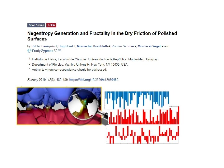
2 FRICCIÓN SECA Y AUTÓMATA CELULAR DE ROBIN HOOD La fricción seca (sin la presencia de un fluido lubricante entre las superficies de cuerpos sólidos en contacto) origina la aparición de una fuerza tangente a las superficies en contacto y opuesta al movimiento o posible movimiento de los cuerpos, esta fuerza recibe el nombre de fuerza de fricción. Macroscópicamente: Tribology is the science and engineering of interacting surfaces in relative motion. It includes the study and application of the principles of friction, lubrication, and wear. Tribology is highly interdisciplinary, drawing on many academic fields, including physics, chemistry, materials science and engineering.

Space tribology is a subset of the lubrication field dealing with the reliable performance of satellites and spacecraft. Historically, the lubricants for space mechanisms have been chosen on the basis of space heritage rather than on the latest technology or the best available materials. Early in the space program, this strategy almost always paid off because mission lifetimes and mechanism duty cycles were minimal. … other spacecraft components, such as, electronics, batteries and computers failed before the lubrication systems. However, in the last decade the tribological systems have become the limiting factor in spacecraft reliability and performance. A classic example was the Galileo spacecraft. Galileo was launched from the Space Shuttle Atlantis in 1989. One of the most important components was a high gain, umbrella like antenna that was closed during launch to conserve space. In 1991 this antenna only partially unfurled. It was concluded that some ribs were stuck in place. Y el reporte explica que: lubricated with a bonded dry film lubricant, had seized due to loss of the lubricant.

Desde un punto de vista microscópico (nanoscópico) la fricción seca se puede entender de la siguiente manera:

We consider sites i in one dimension (1≤i≤N) and consider "heights" hi at each site. The Robin Hood algorithm searches for the maximum height, subtracts a random amount r in [0, 1] from that location, and distributes this amount evenly between the next near neighbors. I. e. , at each time step t the site m with maximal height hm(t)=max{hi(t)} is found and the new heights are determined according to the following rule: A typical snapshot of the steady state is: The maximum height and its "rich" neighborhood are clearly seen at around site 650. Besides a unique singularity, the heights are drastically cut off at heights above hc≈0. 1, the critical height. This can be seen better from the height distribution: there is a wide distribution of heights below hc, while above hc the distribution drops rapidly, hc

To quantitatively analyze the profile generated by the RH algorithm we introduced different metrics. Aquí contaremos una que hemos visto es de interés en el estudio de los autómatas celulares para caracterizarlos • The Shannon’s entropy: More specifically, we consider the change in entropy ΔS with respect to the initial uniformly random surface: Esta métrica la habían utilizado Zypman et al. anteriormente para caracterizar muestras de materiales sometidos a fricción seca. Vamos a utilizar un procedimiento similar al que utilizaron ellos para caracterizar el perfil generado por el AC Robin Hood. So we consider h. T, a threshold height, which controls the asperity interaction range, by whether or not hi>h. T.

La altura del umbral, h. T, es inversamente proporcional a la carga externa, un factor muy relevante en la fricción seca. This threshold is chosen such that: a) h. T ≤ hc 0. 1 since for h. T ≥ hc 0. 1 there are too few points. b) On the other hand, ‘no threshold’ is equivalent to h. T →−∞ (in the infinite limit), although in practice it is enough h. T ≤− 0. 2. Therefore, − 0. 2 ≤. h. T ≤ hc So we compute the entropy by taking into account only the heights h. T. Each measure in the figure was taken every thousand steps, In total 100 M steps. A clear downward trend is seen; saturation at steady state is found after a transient of about 70 million time steps

3. DIFERENTES AC PARA El LONG TERM EVOLUTIONARY EXPERIMENT(LTEE) El LTEE comenzó hace 33 años, en 1988. Dos variantes de e. coli con fenotipos que permiten distinguirlas pero no le dan ninguna ventaja de fitness: A) Una forma colonias blancas. B) La otra forma colonias rojas. Cualquiera de las dos en un cultivo condiciones específicas se duplican cada 3. 6 horas o sea hay 6. 7 generaciones por día = 6. 7× 365 2400 generaciones por año Se llevan registros a lo largo de los 33 años ( 75. 000 generaciones) de 12 poblaciones originadas en una única célula. En 6 se deja sin evolucionar la variante A) y se la compara con la B cada 500 generaciones (500/6. 7 =75 días) durante un día, se llaman experimentos Ara-. En las otras 6 se deja sin evolucionar la variante B) y se la compara con la A c/500 gener, Ara+. Al final de ese día de competencia se mide el número de colonias blancas y rojas y se usa este dato para calcular el fitness de la variante evolucionada relativa al ancestro. En los Ara- el ancestro es blanco (rojo en Ara+) y el evolucionado los es rojo (blanco en Ara+)

En 6. 67 replicaciones la población aumenta en un factor 26. 67 = 100

Para calcular el fitness relativo de la bacteria evolucionada respecto al ancestro al final del día de competencia se mide el número de colonias blancas y rojas y se usa este dato para calcular el fitness de la variante evolucionada relativa al ancestro usando: è The LTEE provides a simple and compelling demonstration of the fact that adaptation by natural selection occurs. The figure shows the step-like fitness trajectory measured for one of the LTEE populations over the course of the first 2, 000 generations of the experiment. [from Lenski and Travisano, 1994, Proc. Natl. Acad. Sci. USA]. Noten que la evolución no es monótona. La población “explora” el paisaje de fitness (subidas y bajadas).

We considered a one-dimensional CA. On each of the N cells we have the fitness fi of an individual. Initial condition: In order to emulate the experimental condition that each of the 12 populations was initiated by a single cell from an asexual clone, we start with the same fitness for all cells, fi = 0. 5 i. The update rule to emulate evolution is as follows. at each time step t we perform the following operations: (a) We eliminate the cell with the lowest fitness. (b) We also eliminate, on average, Q other cells both neighbors of the cell with minimum fitness and with probability p another cell at random; thus Q = 2+p (c) replace the fi associated to the cells eliminated by random numbers generated with a uniform distribution in the interval 0, 1. �: N=1500, Q = 2. 2

20 años no es nada… O si? What We’ve Learned about Evolution from the LTEE: 2. The discovery that fitness can increase “forever” – or at least for a very long time – by adaptation, even in a constant environment. An exciting new twist on the dynamics of adaptation by natural selection is the discovery that fitness can increase “forever” – or at least for a very long time – even in a constant environment. Originalmente (cuando iban 10. 000 generaciones se pensó que el relative fitness había alcanzado una asíntota y que el mejor ajuste lo daba un fit hiperbólico Luego (con 50. 000 o 60. 000 generaciones) se vió que el sistema no ha alcanzado una asíntota: A power-law model, which has no upper bound, gives a significantly better fit to the meanfitness trajectories measured in the LTEE populations: The figure shows the grand-mean fitness data (symbols with error bars) over 50, 000 generations of the LTEE. It also shows the trajectories predicted by the power law (blue curve) and by a model with an asymptote (red curve) using only the first 20, 000 generations of data. [from Wiser et al. , 2013, Science]

What We’ve Learned about Evolution from the LTEE: 5. We have seen large changes in the spontaneous mutation rate in some of the LTEE populations. These changes reflect an interesting tradeoff between short-term fitness and long-term evolvability. The biochemical)causes of these changes are mutations in genes whose products are involved in DNA repair or the degradation of molecules that cause damage to DNA. Hypermutators: Ara-1, Ara-2, Ara-3, Ara-4; Ara+3, Ara+6. No hypermutators: Ara-5, Ara-6; Ara+1, Ara+2; Ara+4, Ara+5.

× 104 generations Wrong! Opposite behavior when the mutation rate increases.

Entonces hemos comenzado a analizar otros autómatas o algoritmos para reproducir, explicar y predecir el LTEE Los parámetros que tenemos para jugar son: N ( manteniendo m constante) f 0: fuerte dependencia, RF∞ 1/ f 0 y la concavidad del inicio

Gracias

FRACTAL DIMENSION In accordance with the computation of the entropy, we must discard all the heights below h. T. Esto plantea la cuestión de, al perder puntos de la curva, como completarla para calcular su dimensión fractal. Probamos con dos procedimientos diferentes y dan resultados muy similares. Hence, A) we replace these heights by hi = h. T, i. e. drawing horizontal lines at height h. T, B) or by first-order interpolation, i. e. by drawing lines between all points remaining (as expected) Linear Interpolation of surface profile.

Then, using the box counting method, we compute the fractal dimension of the resulting “effective” profile. Specifically, we cover the profile with boxes of side e, and find how the number of boxes N changes with e. The fractal dimension of a set S is given then by: For a power law N(e) = 1/e DF, DF is the fractal dimension. To test the box-counting method, we used them on: i) A straight line of constant height 0. 1234567. For this line we got a dimension DF =0. 9998 i. e. an error of 2/10000, ii) The area under this line, and the method produced a DF =1. 986, i. e. an error of 0. 14 %.

We obtained that after a transient of few millions of iterations, the fractal dimension oscillates around DF 1. 56 for. Similar patterns were found for other threshold values greater than 0. Problema AC d Área Segregación racial Schelling 1971 2 Economía Fricción seca Robin Hood 1 Física de Materiales 1 Evolución biológica en tiempo real Long Term Evolution Experiment (LTEE) Bak-Sneppen, Otros

Resumen RH ØUsamos un CA unidimensional para estudiar numéricamente la aproximación al estado estacionario en fricción seca. ØA partir de un perfil de superficie generado aleatoriamente correspondiente a separaciones locales aleatorias entre las superficies de fricción, introdujimos una dinámica basada en el algoritmo de Robin Hood. ØEsto genera un perfil de superficie dependiente del tiempo. ØEse perfil se analizó mediante el cálculo de su contenido de entropía; tanto en función del tiempo como de la altura umbral h. T. que es un proxi de la carga externa. ØEl contenido de entropía se estudió para evaluar la afirmación de que la fricción reduce la entropía. ØResultado que comprobamos. ØDescubrimos que este es el caso en nuestro modelo para todos los h. T; es decir, independientemente de la carga externa, nuestro modelo sugiere una autocuración a través de la fricción. Además, encontramos que el valor de estado estable de la entropía disminuye con h. T o, de manera equivalente, aumenta con la carga externa. Esto se debe al hecho de que a medida que aumenta la carga, las dos superficies se vuelven más íntimamente en contacto y se vuelven detectables imperfecciones más pequeñas.