Announcements Last lecture Tonight 5 6 ARTS Main

Announcements • Last lecture Tonight 5 -6 ARTS Main LT • Thursday 9 -10 Muirhead Main LT: Fazeer Exercise Class on Production Work. Sheet • Marks on Test 2 hopefully by Friday • CORRECT Version of Solution to Test 2 on Network (some minor 1 am errors in original)

Tests in Last Week • 201 Test 3 on Production Worksheet – Monday 11 th Dec 5 -6 Vaughan Jeffries – see final previous years • 201 TFU Final – Thursday 14 th Dec 5 -6 Vaughan Jeffries – see final previous years • 203 Final (Two essays) – Wednesday 13 th 12 -1 Vaughan Jeffries • Will meet in Semester 2 to review test procedure

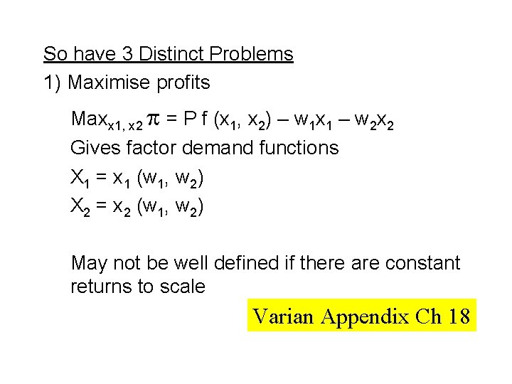
So have 3 Distinct Problems 1) Maximise profits Maxx 1, x 2 p = P f (x 1, x 2) – w 1 x 1 – w 2 x 2 Gives factor demand functions X 1 = x 1 (w 1, w 2) X 2 = x 2 (w 1, w 2) May not be well defined if there are constant returns to scale Varian Appendix Ch 18

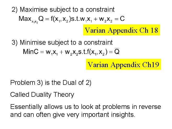
2) Maximise subject to a constraint Varian Appendix Ch 18 3) Minimise subject to a constraint Varian Appendix Ch 19 Problem 3) is the Dual of 2) Called Duality Theory Essentially allows us to look at problems in reverse and can often give very important insights.

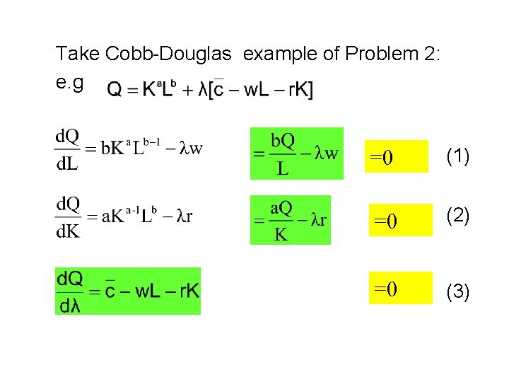
Take Cobb-Douglas example of Problem 2: e. g =0 (1) =0 (2) =0 (3)

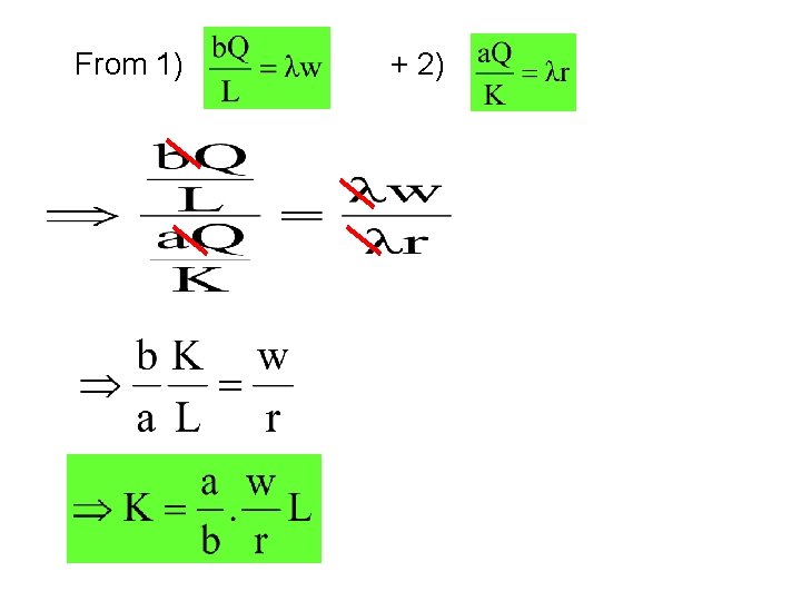
From 1) + 2)

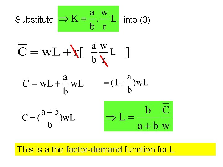
Substitute into (3) This is a the factor-demand function for L

Strictly it is a Cost-constrained factordemand function

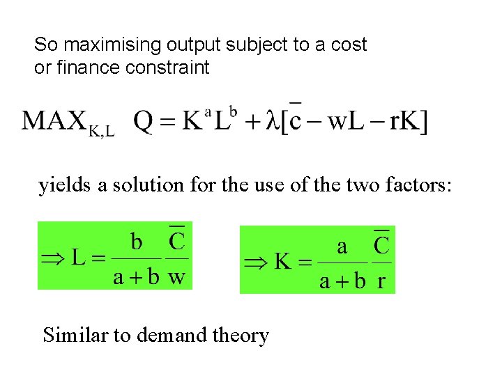
So maximising output subject to a cost or finance constraint yields a solution for the use of the two factors: Similar to demand theory

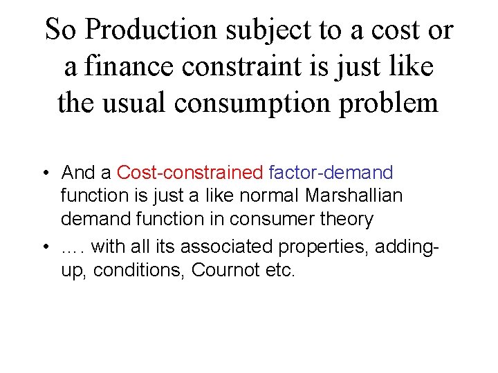
So Production subject to a cost or a finance constraint is just like the usual consumption problem • And a Cost-constrained factor-demand function is just a like normal Marshallian demand function in consumer theory • …. with all its associated properties, addingup, conditions, Cournot etc.

But what about the third problem… That of minimising cost subject to an output constraint? • Again we will work through a Cobb-Douglas example to give you a flavour of the story.

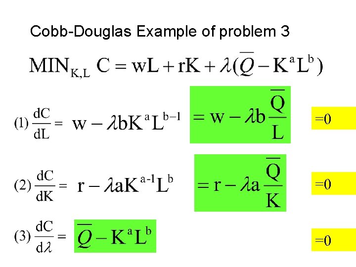
Cobb-Douglas Example of problem 3 =0 =0 =0

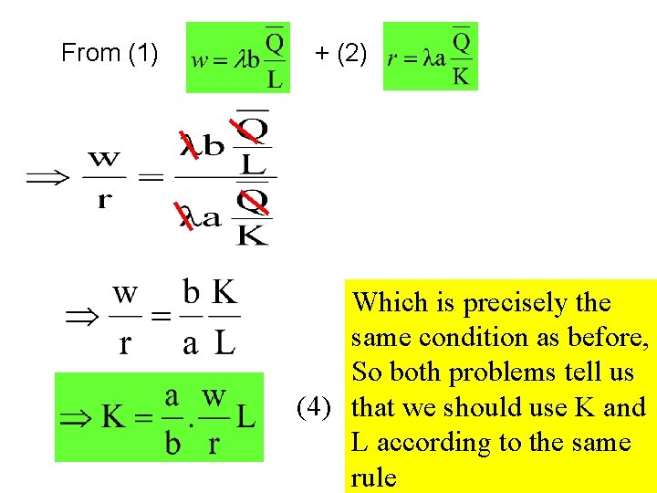
From (1) + (2) Which is precisely the same condition as before, So both problems tell us (4) that we should use K and L according to the same rule

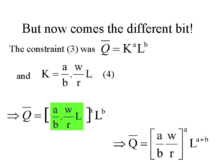
But now comes the different bit! The constraint (3) was and (4)

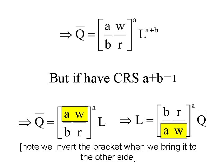
But if have CRS a+b= 1 [note we invert the bracket when we bring it to the other side]

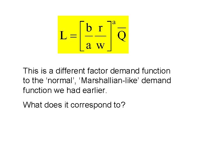
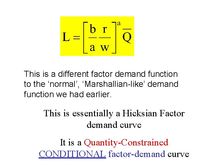
This is a different factor demand function to the ‘normal’, ‘Marshallian-like’ demand function we had earlier. What does it correspond to?

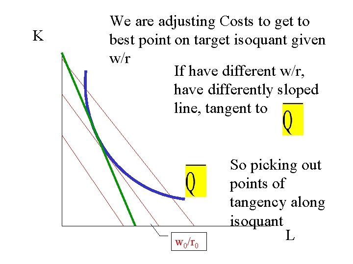
K We are adjusting Costs to get to best point on target isoquant given w/r If have different w/r, have differently sloped line, tangent to w 0/r 0 So picking out points of tangency along isoquant L

This is a different factor demand function to the ‘normal’, ‘Marshallian-like’ demand function we had earlier. This is essentially a Hicksian Factor demand curve It is a Quantity-Constrained CONDITIONAL factor-demand curve

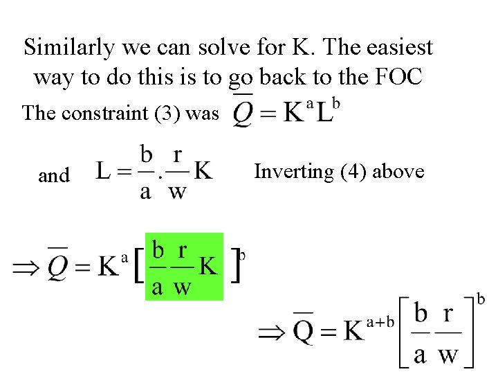
Similarly we can solve for K. The easiest way to do this is to go back to the FOC The constraint (3) was and Inverting (4) above

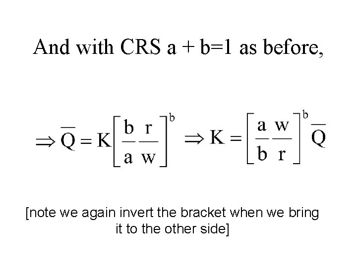
And with CRS a + b=1 as before, [note we again invert the bracket when we bring it to the other side]

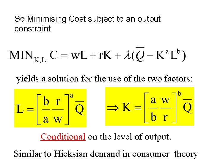
So Minimising Cost subject to an output constraint yields a solution for the use of the two factors: Conditional on the level of output. Similar to Hicksian demand in consumer theory

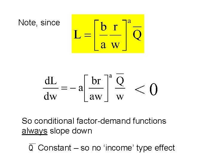
Note, since <0 So conditional factor-demand functions always slope down Constant – so no ‘income’ type effect

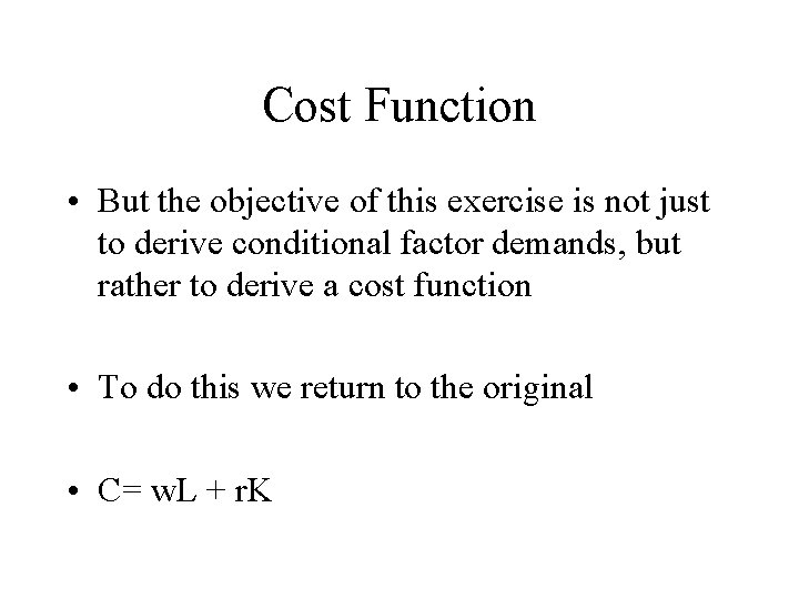
Cost Function • But the objective of this exercise is not just to derive conditional factor demands, but rather to derive a cost function • To do this we return to the original • C= w. L + r. K

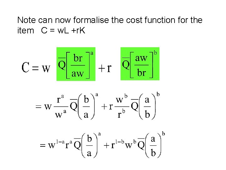
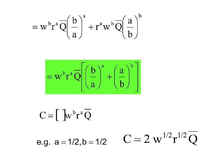
Note can now formalise the cost function for the item C = w. L +r. K

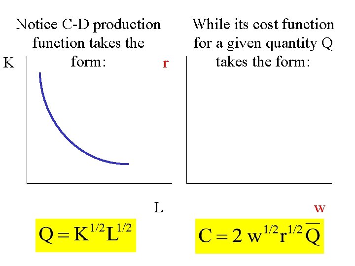
Notice C-D production function takes the form: K r L While its cost function for a given quantity Q takes the form: w

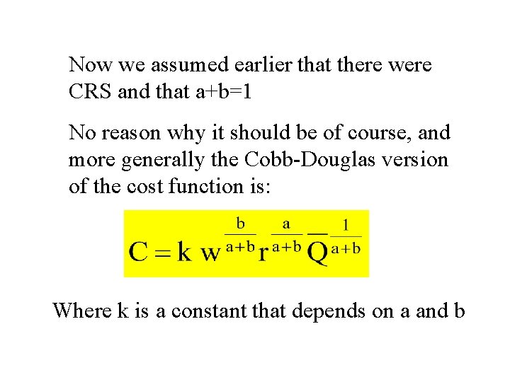
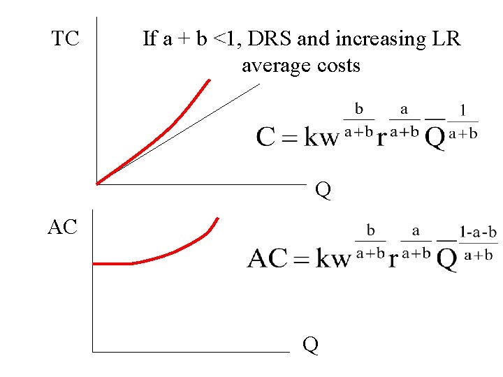
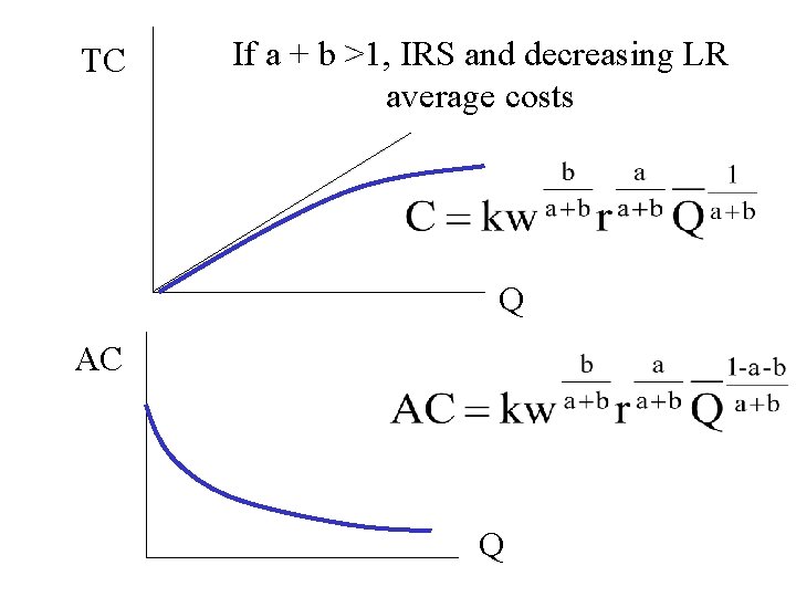
Now we assumed earlier that there were CRS and that a+b=1 No reason why it should be of course, and more generally the Cobb-Douglas version of the cost function is: Where k is a constant that depends on a and b

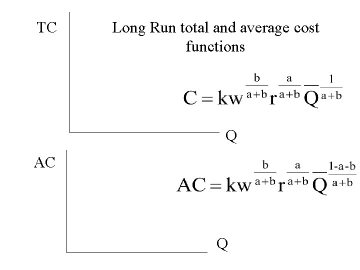
TC Long Run total and average cost functions Q AC Q

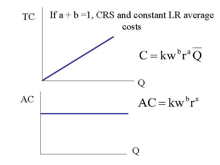
TC If a + b =1, CRS and constant LR average costs Q AC Q

TC If a + b <1, DRS and increasing LR average costs Q AC Q

TC If a + b >1, IRS and decreasing LR average costs Q AC Q

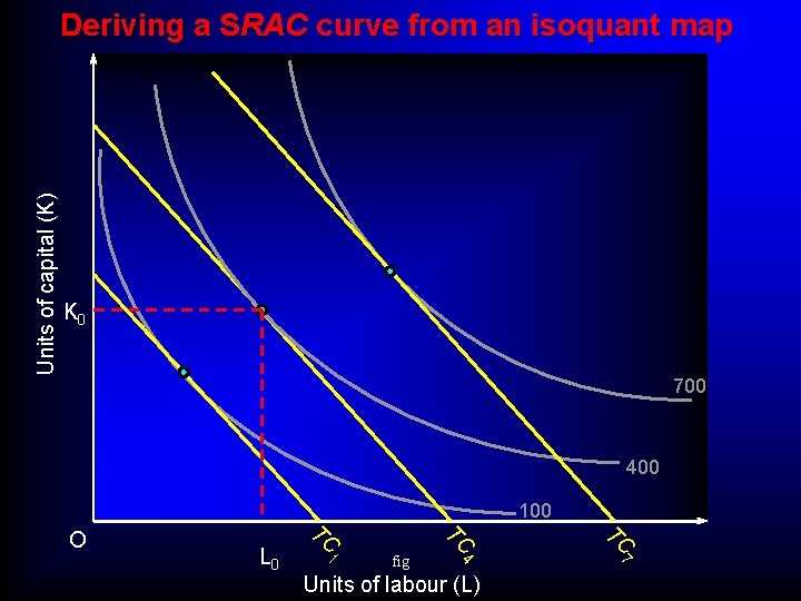
What about the Short-Run? • Derivation of short-run costs from an isoquant map – Recall in SR Capital stock is fixed

Units of capital (K) Deriving a SRAC curve from an isoquant map K 0 700 400 100 TC 4 7 fig TC 1 L 0 TC O Units of labour (L)

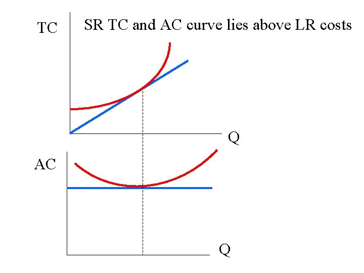
TC SR TC and AC curve lies above LR costs Q AC Q

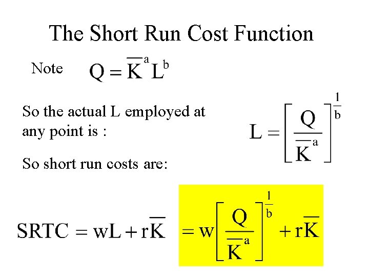
The Short Run Cost Function Note So the actual L employed at any point is : So short run costs are:

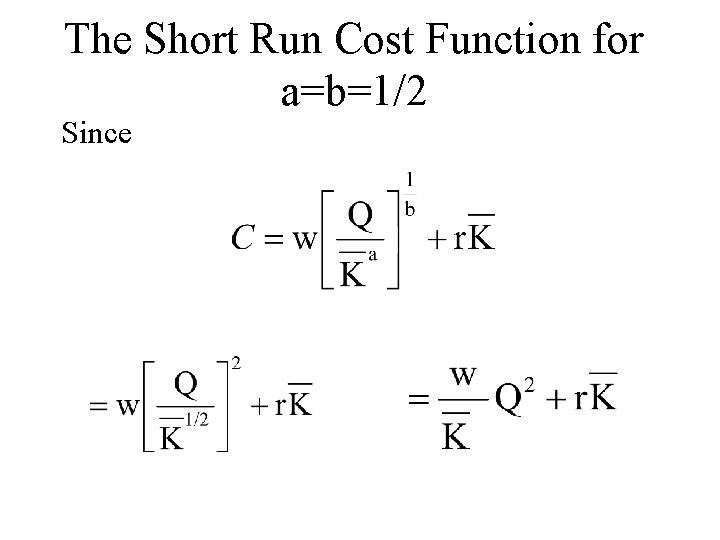
The Short Run Cost Function for a=b=1/2 Since

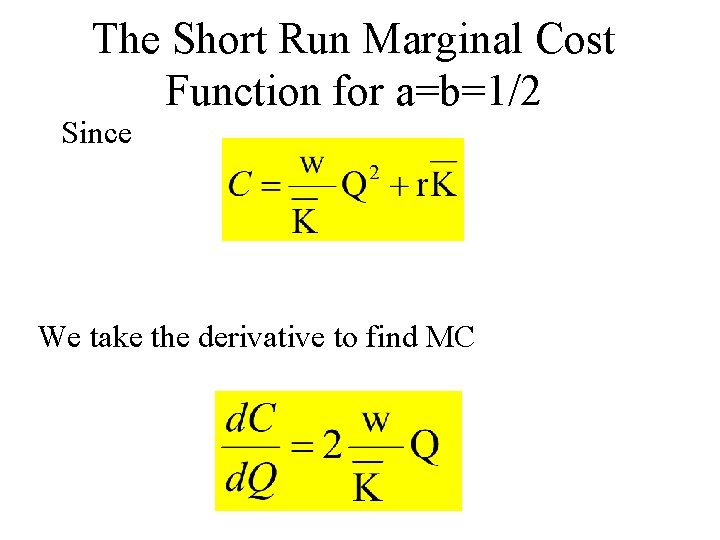
The Short Run Marginal Cost Function for a=b=1/2 Since We take the derivative to find MC

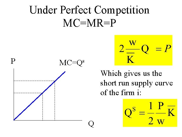
Under Perfect Competition MC=MR=P P MC=Qs Which gives us the short run supply curve of the firm i: Q

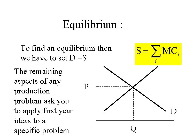
Equilibrium : To find an equilibrium then we have to set D =S The remaining aspects of any production problem ask you to apply first year ideas to a specific problem P D Q

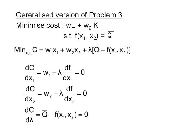
Gereralised version of Problem 3 Minimise cost : w. L + w 2 K s. t. f(x 1, x 2) =

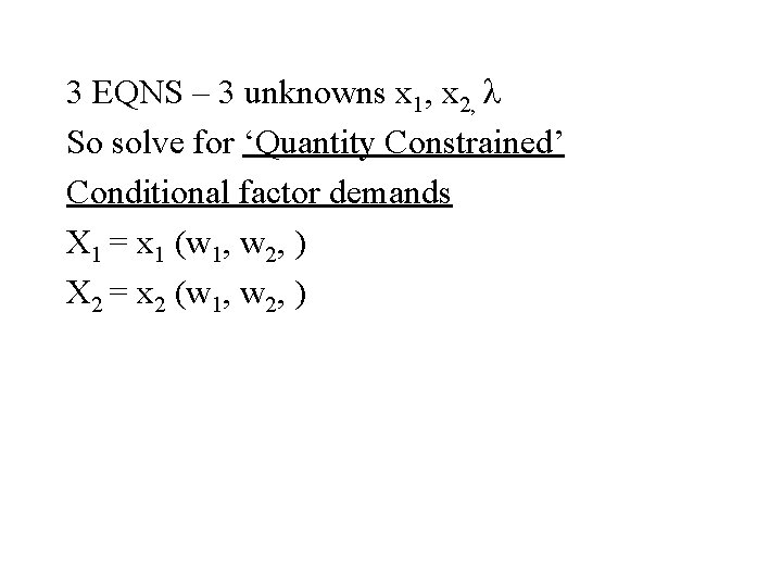
3 EQNS – 3 unknowns x 1, x 2, So solve for ‘Quantity Constrained’ Conditional factor demands X 1 = x 1 (w 1, w 2, ) X 2 = x 2 (w 1, w 2, )