Algorithmic Differentiation in R using the Rcpp Eigen

‘Algorithmic Differentiation in R using the Rcpp. Eigen. AD package’ by Rob Crouchley, Dan Grose, Damon Berridge 1

Motivation • The primary advantage of AD is to eliminate the need to write code for derivatives, which means: • • Significantly less time needed to write code for your own research problem Less code means fewer code bugs Derivatives are provided to machine precision Out performs finite difference methods if dimensionality is large • In statistics AD enables easy application of: • Optimization • The delta method • Implicit function theorem 2

What is Rcpp. Eigen. AD? Rcpp. Eigen. AD Rcpp Multivariate Faà di Bruno, source. Cpp. AD, J, H Marshalling of R data, source. Cpp Eigen Linear Algebra Cpp. AD Algorithmic Differentiation 3

What does Rcpp. Eigen. AD do? • 4

Simple Illustration of Rcpp. Eigen. AD, part 1 Algebra R solve(X) det(X) det(solve(X)) Rcpp. Eigen. AD f<-source. Cpp. AD(' ADmat f(const ADmat& X) {return X. inverse(); }') Rcpp. Eigen. AD f<-source. Cpp. AD(' ADmat f(const ADmat& X) {return X. inverse(); }') g<-source. Cpp. AD(' ADmat g(const ADmat& X) {ADmat res(1, 1); res(0, 0) = X. determinant(); return res; }') not needed 5

Simple Illustration of Rcpp. Eigen. AD, part 2 Recall Algebra Jacobian Hessian 6

Illustration, R results for a 2 by 2 matrix, part 1 > X<-matrix(c(1, 2, 3, 4), 2, 2) > f(X) [, 1] [, 2] [1, ] -2 1. 5 [2, ] 1 -0. 5 > g(X) [, 1] [1, ] -2 > > (g%. %f)(X) [, 1] [1, ] -0. 5 > # The inverse # The determinant of the inverse 7

Illustration, R results for a 2 by 2 matrix, part 2 > J(f)(X) # Jacobian of the inverse [nxn] [, 1] [, 2] [, 3] [, 4] [1, ] -4. 0 2. 0 3. 00 -1. 50 [2, ] 3. 0 -1. 0 -2. 25 0. 75 [3, ] 2. 0 -1. 00 0. 50 [4, ] -1. 5 0. 75 -0. 25 > H(f)(X) # Hessian of the inverse [nxn 2] [, 1] [, 2] [, 3] [, 4] [, 5] [, 6] [, 7] [, 8] [, 9] [, 10] [, 11] [, 12] [, 13] [1, ] -16 8. 0 12. 00 -6. 00 12. 00 -5. 00 -9. 00 3. 75 8. 0 -4 -5. 00 2. 50 -6. 00 [2, ] 8 -4. 0 -5. 00 2. 50 -5. 00 2. 00 3. 00 -1. 25 -4. 0 2 2. 00 -1. 00 2. 50 [3, ] 12 -5. 0 -9. 00 3. 75 -9. 00 3. 00 6. 75 -2. 25 -5. 0 2 3. 00 -1. 25 3. 75 [4, ] -6 2. 5 3. 75 -1. 50 3. 75 -1. 25 -2. 25 0. 75 2. 5 -1 -1. 25 0. 50 -1. 50 [, 14] [, 15] [, 16] [1, ] 2. 50 3. 75 -1. 50 [2, ] -1. 00 -1. 25 0. 50 [3, ] -1. 25 -2. 25 0. 75 [4, ] 0. 50 0. 75 -0. 25 8

Illustration, R results for a 2 by 2 matrix, part 3 > J(g)(X) # Jacobian of the determinant [1 xn] [, 1] [, 2] [, 3] [, 4] [1, ] 4 -2 -3 1 > H(g)(X) # Hessian of the determinant [n 2 xn 2] [, 1] [, 2] [, 3] [, 4] [1, ] 0 0 0 1 [2, ] 0 0 -1 0 [3, ] 0 -1 0 0 [4, ] 1 0 0 0 > J(g%. %f)(X) # Jacobian of the determinant of the inverse [1 xn 2] [, 1] [, 2] [, 3] [, 4] [1, ] -1 0. 5 0. 75 -0. 25 > H(g%. %f)(X) # Hessian of the determinant of the inverse [nxn] [, 1] [, 2] [, 3] [, 4] [1, ] -4. 00 2. 00 3. 00 -1. 25 [2, ] 2. 00 -1. 25 0. 50 [3, ] 3. 00 -1. 25 -2. 25 0. 75 [4, ] -1. 25 0. 50 0. 75 -0. 25 9

Functional decomposition of a statistical model 1. Data, design matrix, transformations 2. Model, a function of the data 3. Log-Likelihood, a function of the Model and the Data • We can obtain any cross derivatives of the parts and their components via Faà di Bruno's formula (an identity which generalizes the chain rule to higher order derivatives) 10

Statistical Model Applications: 1. model estimation (using the 1 st and 2 nd derivatives to maximize a function) 2. model interpretation (the delta method is used to produce SE of the model’s marginal effects) 3. model criticism (the implicit function theorem is used to check for the model’s internal validity) On a logit model of the Finney (1971) data. 11

The Finney (1971) experimental data, n=39 • 12

Example 1. max. Lik with AD for the J and H gives Maximum Likelihood estimation Newton-Raphson maximisation, 6 iterations Return code 1: gradient close to zero Log-Likelihood: -14. 61369 3 free parameters Estimates: Estimate Std. error theta 1 -2. 875 1. 321 # constant theta 2 5. 179 1. 865 # ln(Vol) theta 3 4. 562 1. 838 # ln(Rate) Same as the result give by max. Lik with analytical derivatives, using AD we can easily do this for any model with a couple of lines of R code 13

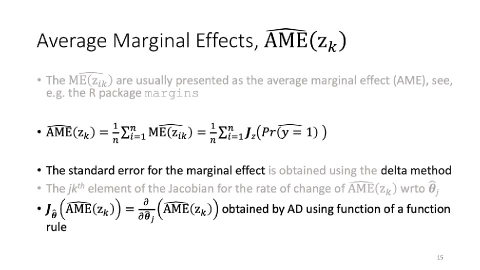
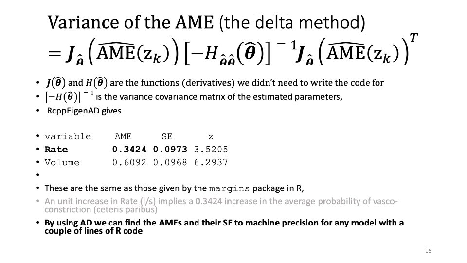
Example 2: Rcpp. Eigen. AD and model Interpretation • 14

Example 3: Using Rcpp. Eigen. AD for model criticism • Influence statistics provide a measure of the stability of the model’s outputs with respect to the data components, they can indicate the degree of change in the model outputs when a data point/case (or group of cases) is dropped • This could be important if some elements of the data set have been corrupted or if the model is not appropriate for a subset of the data • There are many tools that can be used to detect influential observations, e. g. Cook’s D, DFBETAs, DFFITs, and Studentized Residuals • We only consider the role of Rcpp. Eigen. AD for DFBETAs 17

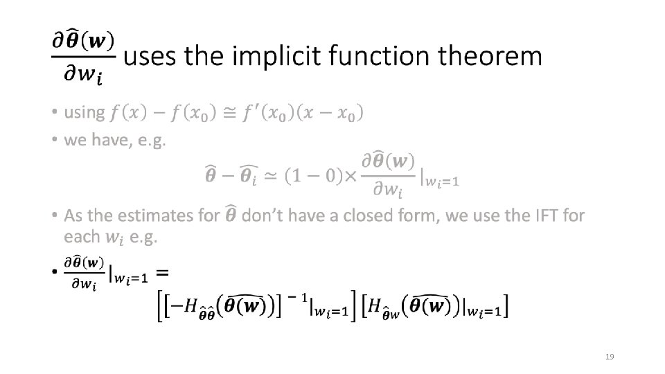
Infinitesimal Influence • 18

Infinitesimal Influence: DFBETA • 20

Infinitesimal Influence: DFBETAs Example 21

Infinitessimal Influence: Example • 22

Summary • Rcpp. Eigen. AD has eliminated the need to write code for derivatives • Rcpp. Eigen. AD means statistical modellers have the tools to help with; • estimation • Interpretation • sensitivity analysis of any model new or otherwise • Which could imply better science in less time • Different components (i. e. not data, model, estimation) could be used in other areas e. g. data reduction 23