Advance Analysis of Algorithms Lecture 8 Growth of

Advance Analysis of Algorithms Lecture 8 Growth of Functions - Asymptotic Notations

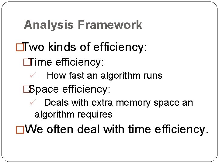
Analysis Framework �Two kinds of efficiency: �Time efficiency: ü How fast an algorithm runs �Space efficiency: ü Deals with extra memory space an algorithm requires �We often deal with time efficiency.

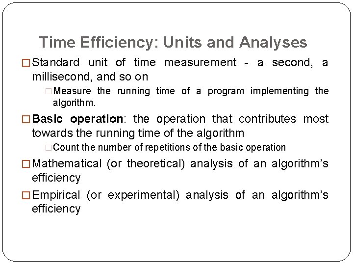
Time Efficiency: Units and Analyses � Standard unit of time measurement - a second, a millisecond, and so on �Measure the running time of a program implementing the algorithm. � Basic operation: the operation that contributes most towards the running time of the algorithm �Count the number of repetitions of the basic operation � Mathematical (or theoretical) analysis of an algorithm’s efficiency � Empirical (or experimental) analysis of an algorithm’s efficiency

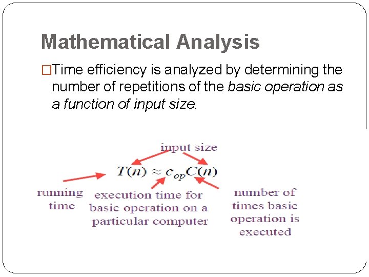
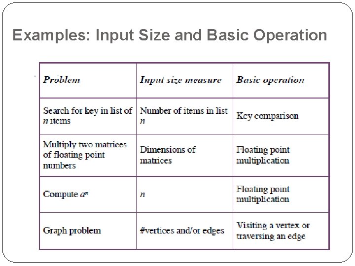
Mathematical Analysis �Time efficiency is analyzed by determining the number of repetitions of the basic operation as a function of input size.

Examples: Input Size and Basic Operation

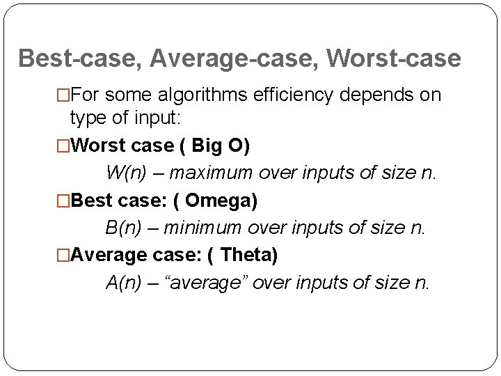
Best-case, Average-case, Worst-case �For some algorithms efficiency depends on type of input: �Worst case ( Big O) W(n) – maximum over inputs of size n. �Best case: ( Omega) B(n) – minimum over inputs of size n. �Average case: ( Theta) A(n) – “average” over inputs of size n.

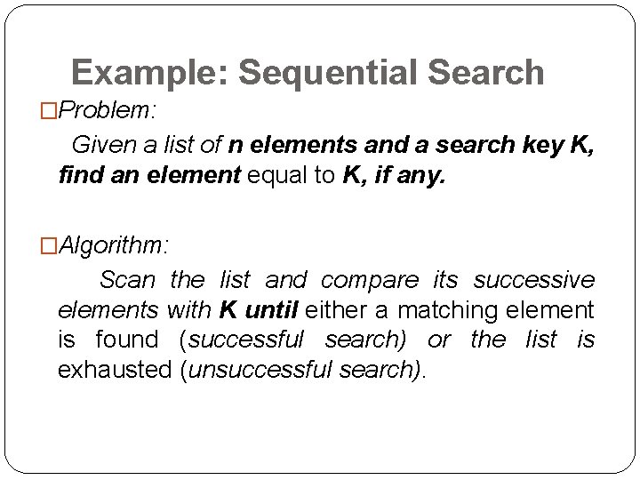
Example: Sequential Search �Problem: Given a list of n elements and a search key K, find an element equal to K, if any. �Algorithm: Scan the list and compare its successive elements with K until either a matching element is found (successful search) or the list is exhausted (unsuccessful search).

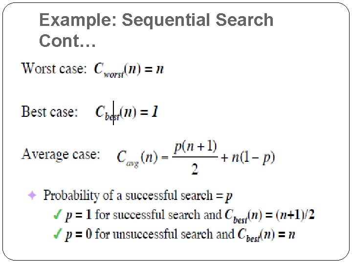
Example: Sequential Search Cont…

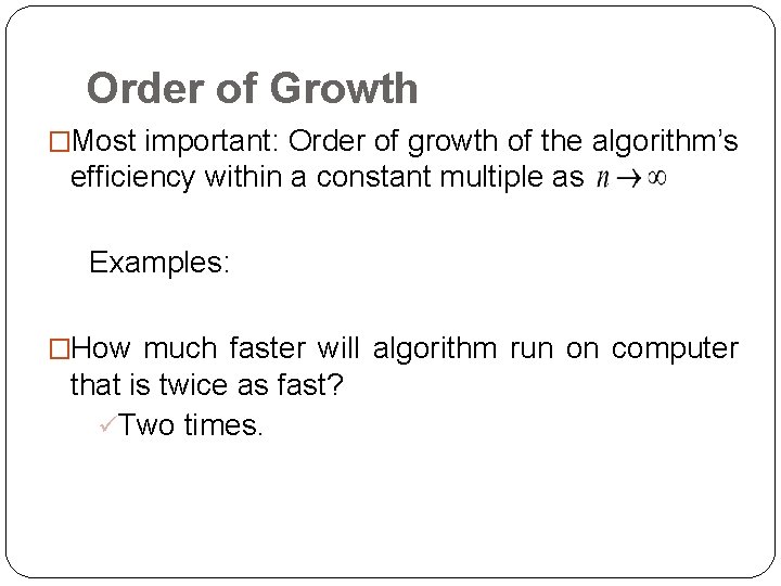
Order of Growth �Most important: Order of growth of the algorithm’s efficiency within a constant multiple as Examples: �How much faster will algorithm run on computer that is twice as fast? üTwo times.

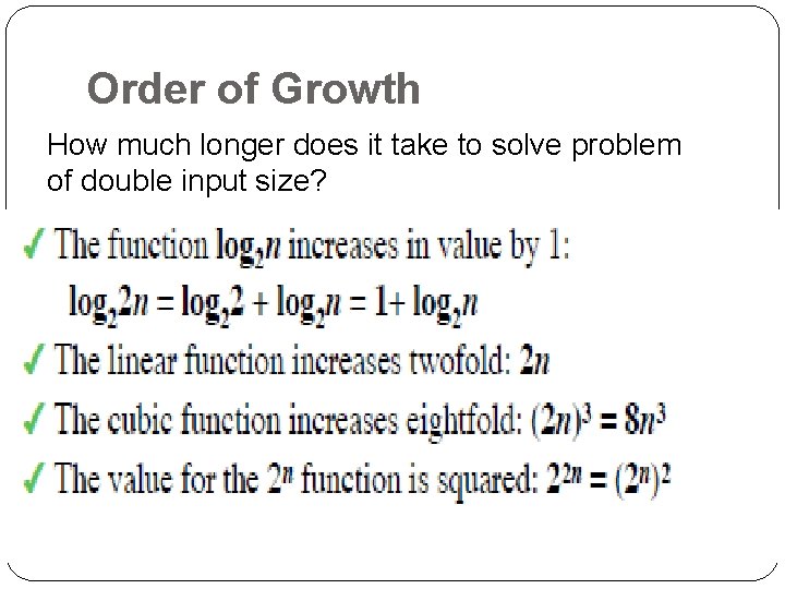
Order of Growth How much longer does it take to solve problem of double input size?

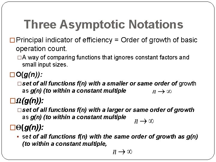
Three Asymptotic Notations � Principal indicator of efficiency = Order of growth of basic operation count. �A way of comparing functions that ignores constant factors and small input sizes. � O(g(n)): �set of all functions f(n) with a smaller or same order of growth as g(n) (to within a constant multiple �Ω(g(n)): �set of all functions f(n) with a larger or same order of growth as g(n) (to within a constant multiple �Ѳ(g(n)): § set of all functions f(n) with the same order of growth as g(n) (to within a constant multiple,

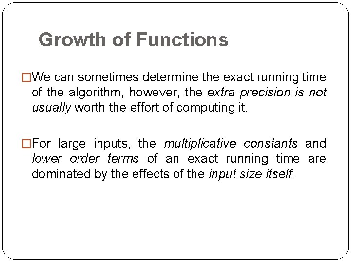
Growth of Functions �We can sometimes determine the exact running time of the algorithm, however, the extra precision is not usually worth the effort of computing it. �For large inputs, the multiplicative constants and lower order terms of an exact running time are dominated by the effects of the input size itself.

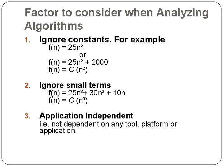
Factor to consider when Analyzing Algorithms 1. Ignore constants. For example, 2. Ignore small terms 3. Application Independent f(n) = 25 n² or f(n) = 25 n² + 2000 f(n) = O (n²) f(n) = 25 n³+ 30 n² + 10 n f(n) = O (n³) i. e. not dependent on any tool, platform or application.

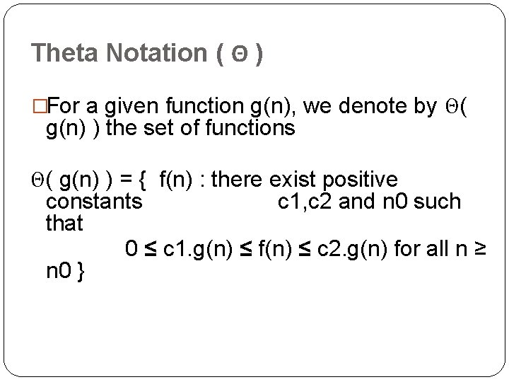
Theta Notation ( Θ ) �For a given function g(n), we denote by Θ( g(n) ) the set of functions Θ( g(n) ) = { f(n) : there exist positive constants c 1, c 2 and n 0 such that 0 ≤ c 1. g(n) ≤ f(n) ≤ c 2. g(n) for all n ≥ n 0 }

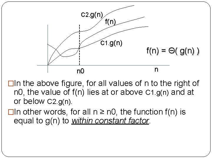
C 2. g(n) f(n) C 1. g(n) f(n) = Θ( g(n) ) n 0 n �In the above figure, for all values of n to the right of n 0, the value of f(n) lies at or above C 1. g(n) and at or below C 2. g(n). �In other words, for all n ≥ n 0, the function f(n) is equal to g(n) to within constant factor.

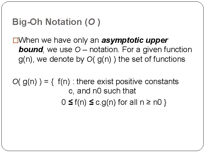
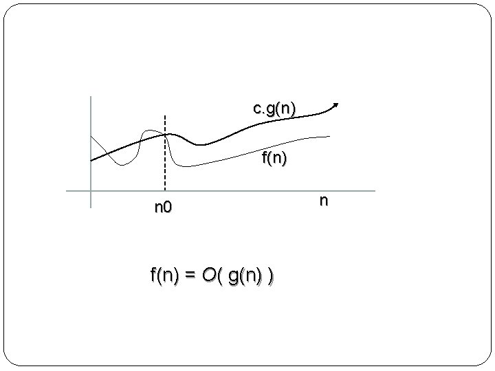
Big-Oh Notation (O ) �When we have only an asymptotic upper bound, we use O – notation. For a given function g(n), we denote by O( g(n) ) the set of functions O( g(n) ) = { f(n) : there exist positive constants c, and n 0 such that 0 ≤ f(n) ≤ c. g(n) for all n ≥ n 0 }

c. g(n) f(n) n 0 f(n) = O( g(n) ) n

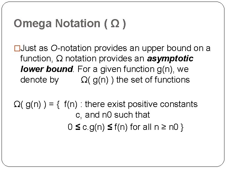
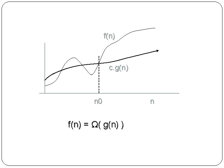
Omega Notation ( Ω ) �Just as O-notation provides an upper bound on a function, Ω notation provides an asymptotic lower bound. For a given function g(n), we denote by Ω( g(n) ) the set of functions Ω( g(n) ) = { f(n) : there exist positive constants c, and n 0 such that 0 ≤ c. g(n) ≤ f(n) for all n ≥ n 0 }

f(n) c. g(n) n 0 f(n) = Ω( g(n) ) n

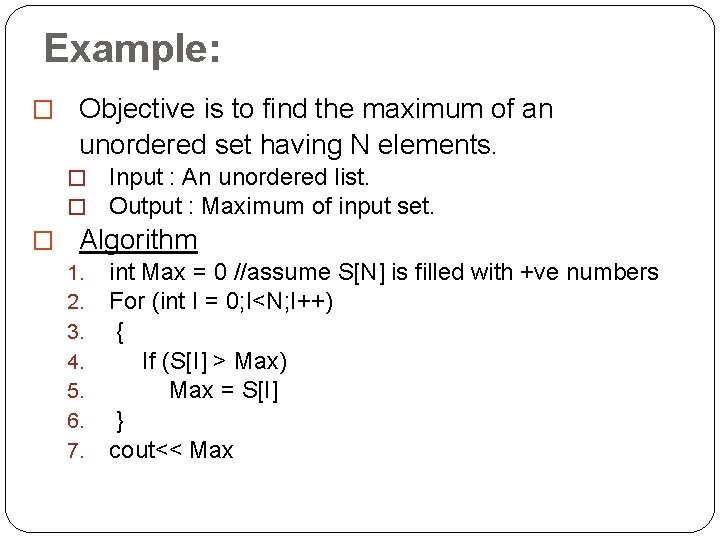
Example: � Objective is to find the maximum of an unordered set having N elements. � � Input : An unordered list. Output : Maximum of input set. � Algorithm 1. int Max = 0 //assume S[N] is filled with +ve numbers 2. For (int I = 0; I<N; I++) 3. { 4. If (S[I] > Max) 5. Max = S[I] 6. } 7. cout<< Max

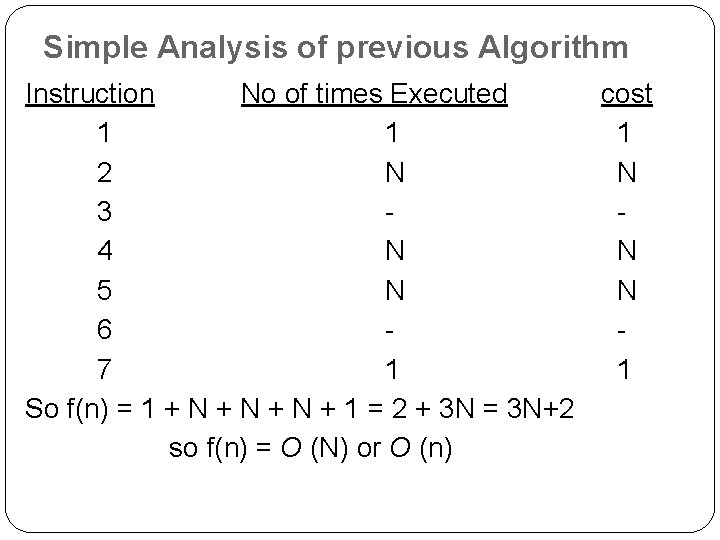
Simple Analysis of previous Algorithm Instruction No of times Executed cost 1 1 1 2 N N 3 4 N N 5 N N 6 7 1 1 So f(n) = 1 + N + N + 1 = 2 + 3 N = 3 N+2 so f(n) = O (N) or O (n)

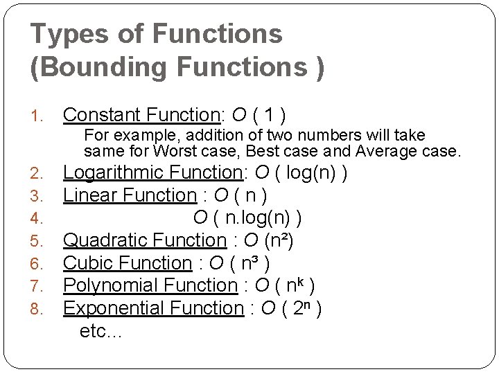
Types of Functions (Bounding Functions ) 1. Constant Function: O ( 1 ) For example, addition of two numbers will take same for Worst case, Best case and Average case. 2. 3. 4. 5. 6. 7. 8. Logarithmic Function: O ( log(n) ) Linear Function : O ( n ) O ( n. log(n) ) Quadratic Function : O (n²) Cubic Function : O ( n³ ) Polynomial Function : O ( nk ) Exponential Function : O ( 2 n ) etc…

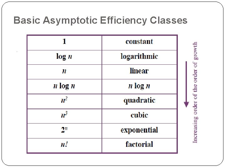
Basic Asymptotic Efficiency Classes

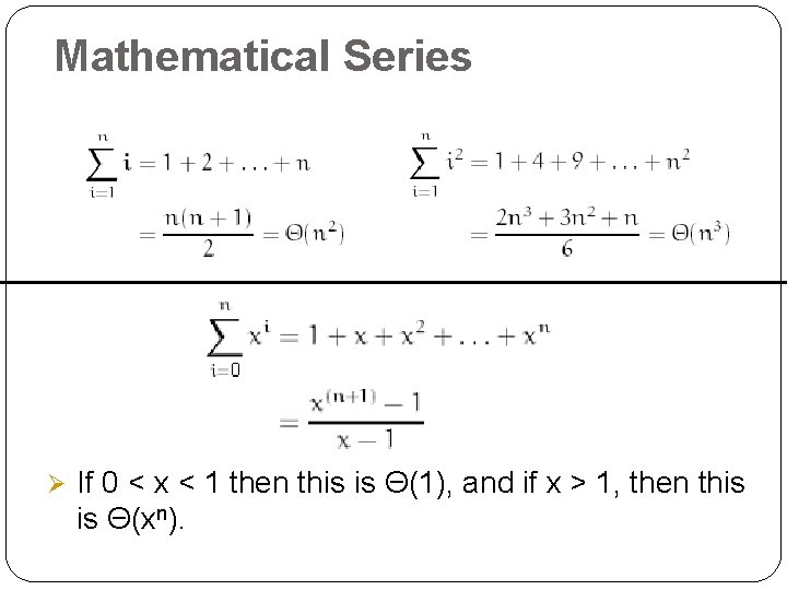
Mathematical Series Ø If 0 < x < 1 then this is Θ(1), and if x > 1, then this is Θ(xn).

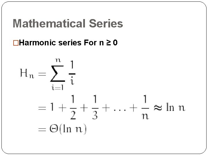
Mathematical Series �Harmonic series For n ≥ 0

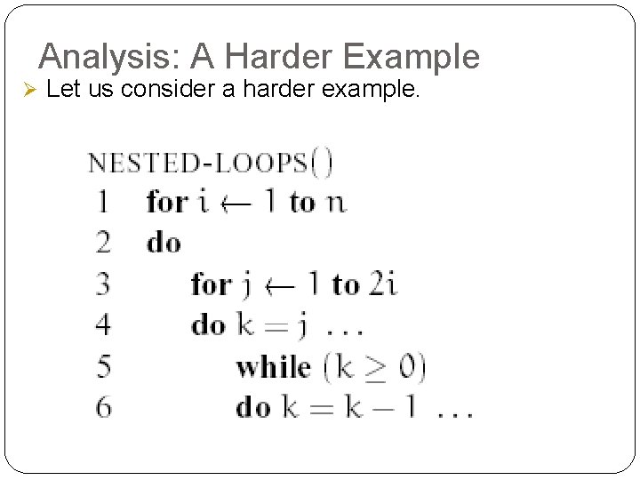
Analysis: A Harder Example Ø Let us consider a harder example.

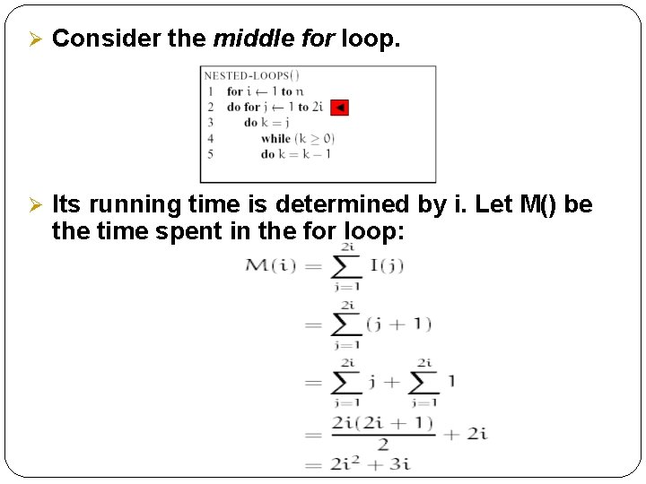
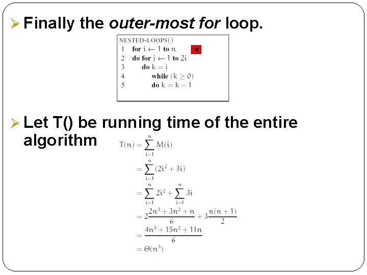
Analysis: A Harder Example Ø How do we analyze the running time of an algorithm that has complex nested loop? Ø The answer is we write out the loops as summations and then solve the summations. Ø To convert loops into summations, we work from inside-out.

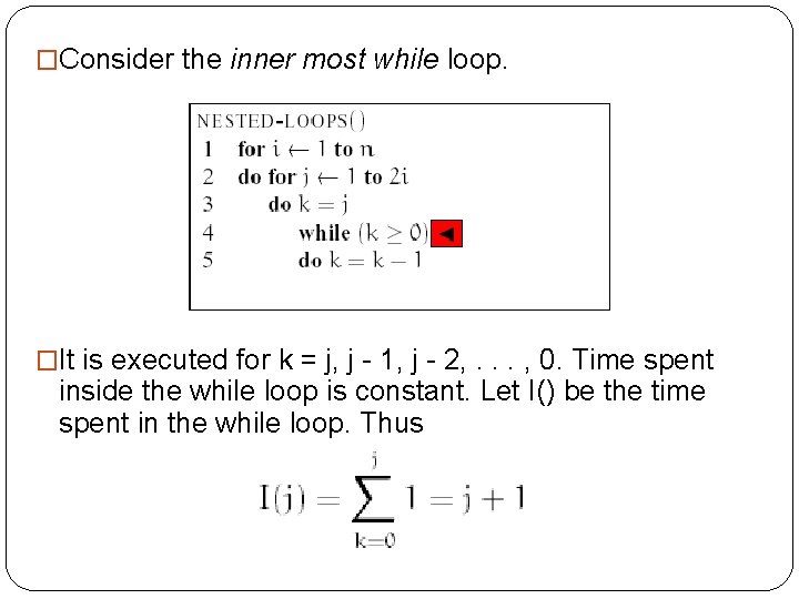
�Consider the inner most while loop. �It is executed for k = j, j - 1, j - 2, . . . , 0. Time spent inside the while loop is constant. Let I() be the time spent in the while loop. Thus

Ø Consider the middle for loop. Ø Its running time is determined by i. Let M() be the time spent in the for loop:

Ø Finally Ø Let the outer-most for loop. T() be running time of the entire algorithm

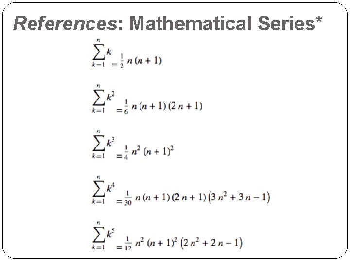
References: Mathematical Series*

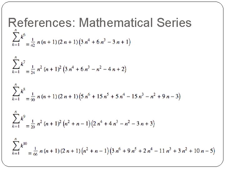
References: Mathematical Series

Empirical Analysis of Algorithms �A complementary approach to mathematical analysis is empirical analysis of an algorithm’s efficiency. �A general plan for the empirical analysis involves the following steps: �Understand the purpose of the analysis process (called experimentation)

Empirical Analysis of Algorithms �Decide on the efficiency metric to be measured and the measurement unit �Decide on characteristics of the input sample �Generate a sample of inputs �Implement the algorithm for its execution (to run computer experiment/simulation) �Execute the program to generate outputs �Analyze the output data.

Analyzing Output Data �Collect and analyze the empirical data (for basic counts or timings) � Present the data in a tabular or graphical form �Compute the ratios M(n)/g(n), where g(n) is a candidate to represent the �efficiency of the algorithm in question n Compute the ratios M(2 n)/M(n) to see how the running time reacts to doubling of its input size

Analyzing Output Data �Examine the shape of the plot: �A concave shape for the logarithmic algorithm �A straight line for a linear algorithm �Convex shapes for quadratic and cubic algorithms �An exponential algorithm requires a logarithmic scale for the vertical axis.