Advance Analysis of Algorithms Lecture 7 1 Quick

Advance Analysis of Algorithms Lecture # 7 1

Quick Sort �It is one of the fastest sorting algorithms known and is the method of choice in most sorting libraries. �Quicksort is based on the divide and conquer strategy. Here is the algorithm: 2

Quicksort A[p…q] ≤ A[q+1…r] � Sort an array A[p…r] � Divide �Partition the array A into 2 subarrays A[p. . q] and A[q+1. . r], such that each element of A[p. . q] is smaller than or equal to each element in A[q+1. . r] �The index (pivot) q is computed � Conquer �Recursively sort A[p. . q-1] and A[q+1. . r] using Quicksort � Combine �The entire array is now sorted 3 CS 477/677 - Lecture 6

QUICK SORT Alg. : QUICKSORT(A, p, r) if p < r then q ← PARTITION(A, p, r) QUICKSORT(A, p, q - 1) QUICKSORT(A, q + 1, r) The pivot is no longer included in any of the subarrays!!

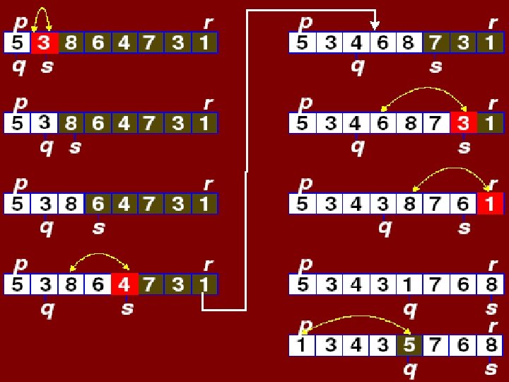
PARTITION(array A, int p, int r) 0. Select Pivot and exchange it to first position of the array 1 2 3 4 5 6 7 8 5 x A[p] q p for s p + 1 to r do if (A[s] < x) then q q + 1 swap A[q] with A[s] swap A[p] with A[q] return q

Example 5 3 8 6 4 7 3 1

Analysis of Quick sort �The running time of quicksort depends heavily on the selection of the pivot. If the rank (index value) of the pivot is very large or very small then the partition (BST) will be unbalanced. �Since the pivot is chosen randomly in our algorithm, the expected running time is O(n log n). �The worst case time, however, is O(n 2). Luckily, this happens rarely. 8

Analysis of Quick Sort �the for loop stops when the indexes cross, hence there are N iterations �swap is one operation – disregarded �Two recursive calls: �Best case: each call is on half the array, hence time is 2 T(N/2) �Worst case: one array is empty, the other is N-1 elements, hence time is T(N-1) �T(N) = T(i) + T(N - i -1) + c. N

Analysis of Quick Sort �The time to sort the file is equal to �the time to sort the left partition with i elements, plus �the time to sort the right partition with N-i-1 elements, plus �the time to build the partitions

T

(Cancel similar terms on both sides)

Analysis of Quick Sort � 2. 1. Worst case analysis � The pivot is the smallest element � T(N) = T(N-1) + c. N , N>1 Telescoping: � T(N-1) = T(N-2) + c(N-1) � T(N-2) = T(N-3) + c(N-2) � T(N-3) = T(N-4) + c(N-3) � T(2) = T(1) + c. 2 Add all equations: T(N) + T(N-1) + T(N-2) + … + T(2) = = T(N-1) + T(N-2) + … + T(2) + T(1) + c(N-1) + c(N-2) + … + c. 2 � T(N) = T(1) + c times (the sum of 2 thru N) = T(1) + c(N(N+1)/2 -1) = O(N 2)

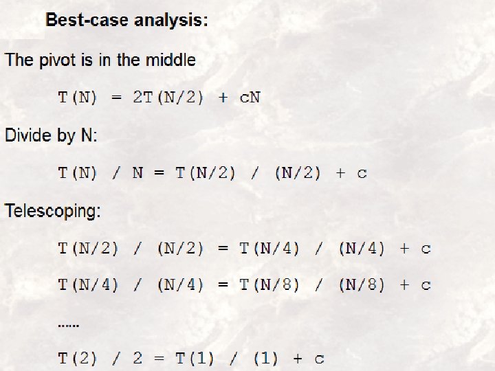
Analysis of Quick Sort � 2. 2. Best-case analysis: � The pivot is in the middle � T(N) = 2 T(N/2) + c. N Divide by N: � T(N) / N = T(N/2) / (N/2) + c Telescoping: � T(N/2) / (N/2) = T(N/4) / (N/4) + c � T(N/4) / (N/4) = T(N/8) / (N/8) + c � …… � T(2) / 2 = T(1) / (1) + c � Add all equations: � T(N) / N + T(N/2) / (N/2) + T(N/4) / (N/4) + …. + T(2) / 2 = � = (N/2) / (N/2) + T(N/4) / (N/4) + … + T(1) / (1) + c. log. N After crossing the equal terms: � T(N)/N = T(1) + c. Log. N � T(N) = N + Nc. Log. N = O(Nlog. N)