851 0585 04 L Modeling and Simulating Social

851 -0585 -04 L – Modeling and Simulating Social Systems with MATLAB Lecture 9 – Scientific Writing and Presentation of Results Karsten Donnay and Stefano Balietti Chair of Sociology, in particular of Modeling and Simulation © ETH Zürich | 2011 -05 -02

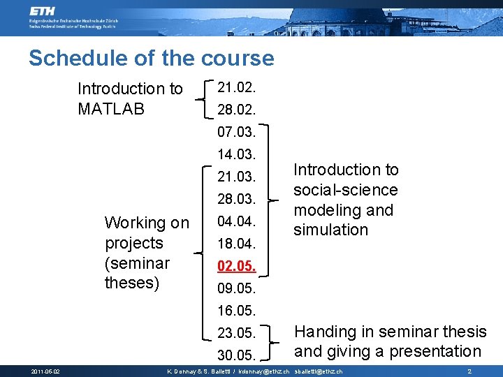
Schedule of the course Introduction to MATLAB 21. 02. 28. 02. 07. 03. 14. 03. 21. 03. 28. 03. Working on projects (seminar theses) 04. 18. 04. Introduction to social-science modeling and simulation 02. 05. 09. 05. 16. 05. 23. 05. 30. 05. 2011 -05 -02 Handing in seminar thesis and giving a presentation K. Donnay & S. Balietti / kdonnay@ethz. ch sbalietti@ethz. ch 2

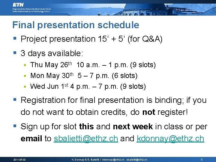
Final presentation schedule § Project presentation 15’ + 5’ (for Q&A) § 3 days available: Thu May 26 th 10 a. m. – 1 p. m. (9 slots) § Mon May 30 th 5 – 7 p. m. (6 slots) § Wed Jun 1 st 4 p. m. – 7 p. m. (9 slots) § § Registration for final presentation is binding; if you do not want to obtain credits, do not register! § Sign up for slot this and next week in class or per email to sbalietti@ethz. ch and kdonnay@ethz. ch 2011 -05 -02 K. Donnay & S. Balietti / kdonnay@ethz. ch sbalietti@ethz. ch 3

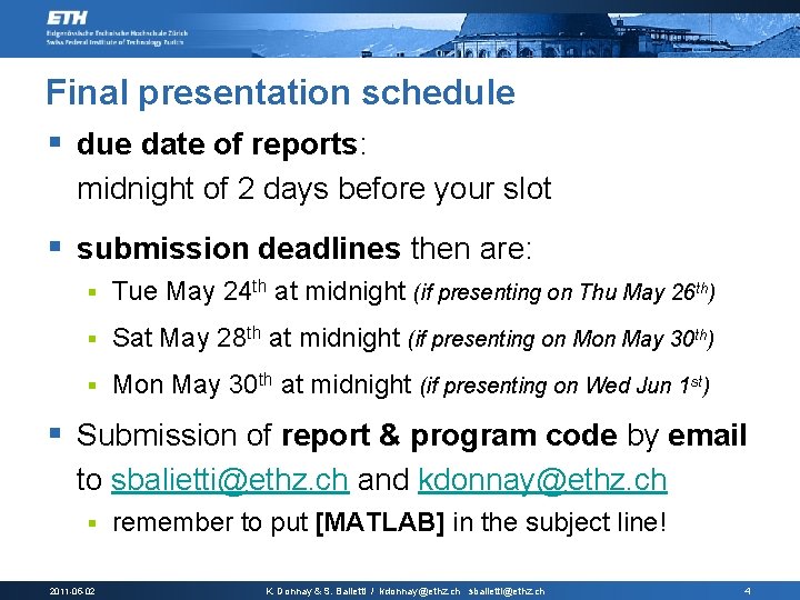
Final presentation schedule § due date of reports: midnight of 2 days before your slot § submission deadlines then are: § Tue May 24 th at midnight (if presenting on Thu May 26 th) § Sat May 28 th at midnight (if presenting on May 30 th) § Mon May 30 th at midnight (if presenting on Wed Jun 1 st) § Submission of report & program code by email to sbalietti@ethz. ch and kdonnay@ethz. ch § 2011 -05 -02 remember to put [MATLAB] in the subject line! K. Donnay & S. Balietti / kdonnay@ethz. ch sbalietti@ethz. ch 4

Goals of Lecture 9: students will 1. Refresh knowledge on optimization in MATLAB acquired in lecture 8, through a brief repetition of important points. 2. Receive a quick introduction to scientific writing* and practical advice on the framing of the final report. 3. Get some specific instructions on the expected format of the final report and a content “checklist” to follow when writing up the report. 4. See an example of the level of sophistication we expect in visualizing your model results. * thanks to Heiko Rauhut and Volker Grimm for providing content 2011 -05 -02 K. Donnay & S. Balietti / kdonnay@ethz. ch sbalietti@ethz. ch 5

Repetition § the structure and simplicity of your code is the most important factor for the performance of your program § make use of the MATLAB specific techniques to improve performance when writing routines; use functions over scripts and compartmentalize § test your program for performance, in particular the parts of your code that carry the main computational load; MATLAB’s profiler is very useful for that! § example of vectorizing: can be faster than looping but not necessarily; the only way to know is to test your program under the expected load of the simulation. § parallelization very easy and useful for parameter sweeps 2011 -05 -02 K. Donnay & S. Balietti / kdonnay@ethz. ch sbalietti@ethz. ch 6

Scientific Writing § Clear, easy to read, concise, and precise. avoid metaphors; use examples instead § keep sentences short § § Main purpose: communicate your work so that others can replicate it, modify it and object to it. § It is still a form of creative writing! create a narrative § guide the reader through your project and results § 2011 -05 -02 K. Donnay & S. Balietti / kdonnay@ethz. ch sbalietti@ethz. ch 7

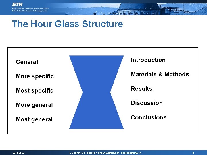
The Hour Glass Structure 2011 -05 -02 K. Donnay & S. Balietti / kdonnay@ethz. ch sbalietti@ethz. ch 8

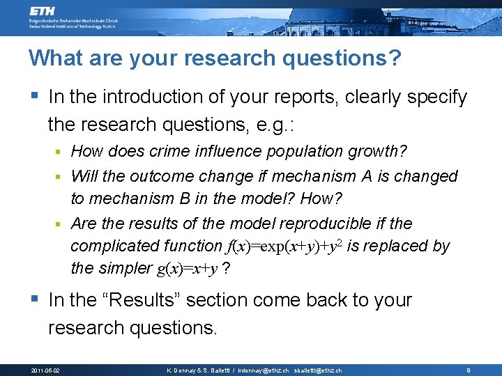
What are your research questions? § In the introduction of your reports, clearly specify the research questions, e. g. : How does crime influence population growth? § Will the outcome change if mechanism A is changed to mechanism B in the model? How? § Are the results of the model reproducible if the complicated function f(x)=exp(x+y)+y 2 is replaced by the simpler g(x)=x+y ? § § In the “Results” section come back to your research questions. 2011 -05 -02 K. Donnay & S. Balietti / kdonnay@ethz. ch sbalietti@ethz. ch 9

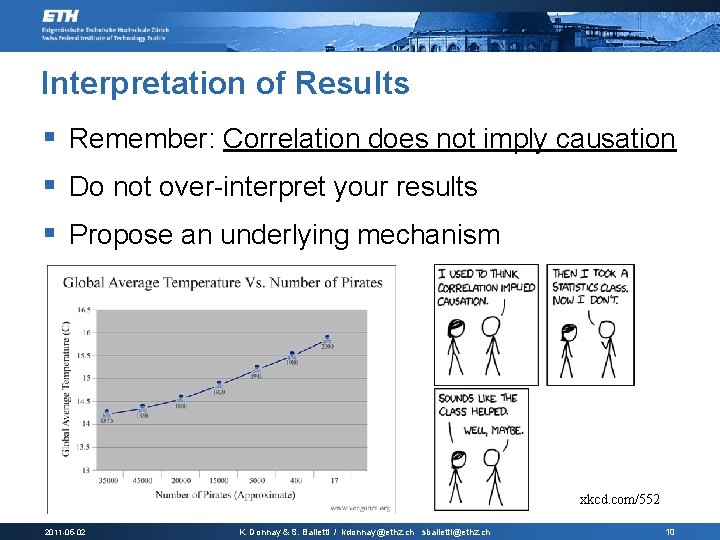
Interpretation of Results § Remember: Correlation does not imply causation § Do not over-interpret your results § Propose an underlying mechanism xkcd. com/552 2011 -05 -02 K. Donnay & S. Balietti / kdonnay@ethz. ch sbalietti@ethz. ch 10

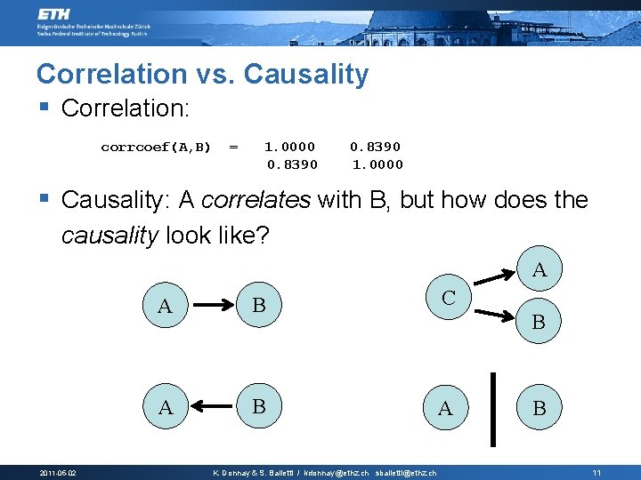
Correlation vs. Causality § Correlation: corrcoef(A, B) = 1. 0000 0. 8390 1. 0000 § Causality: A correlates with B, but how does the causality look like? A 2011 -05 -02 A B C A B A K. Donnay & S. Balietti / kdonnay@ethz. ch sbalietti@ethz. ch B B 11

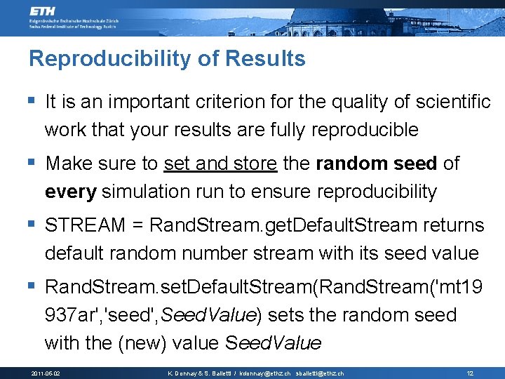
Reproducibility of Results § It is an important criterion for the quality of scientific work that your results are fully reproducible § Make sure to set and store the random seed of every simulation run to ensure reproducibility § STREAM = Rand. Stream. get. Default. Stream returns default random number stream with its seed value § Rand. Stream. set. Default. Stream(Rand. Stream('mt 19 937 ar', 'seed', Seed. Value) sets the random seed with the (new) value Seed. Value 2011 -05 -02 K. Donnay & S. Balietti / kdonnay@ethz. ch sbalietti@ethz. ch 12

Data Dump – storing your results § Make sure that the results of your simulations are stored at the end of a simulation run § You can for example simply save the results in form of the array structure (matrix, cell array) of your simulation using MATLAB’s save() command § Or you may export them to comma separated files using csvwrite() (and csvread() to recover data) § Documentation on csvwrite() may be found here 2011 -05 -02 K. Donnay & S. Balietti / kdonnay@ethz. ch sbalietti@ethz. ch 13

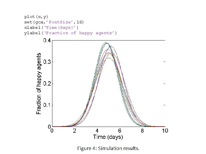
Visualization of Results § Graphical formats: use PDF or EPS in the print version. JPG (better PNG) just for quick visualizations § Increase the font sizes for readability: set(gca, ‘Font. Size’, 16); § ALWAYS use labels on axes: xlabel(‘Time (s)’, ‘Font. Size’, 16); ylabel(‘Number of Agents’, ‘Font. Size’, 16); 2011 -05 -02 K. Donnay & S. Balietti / kdonnay@ethz. ch sbalietti@ethz. ch 14

Visualization of Results (2) § Put a box around the figure: box on § Show grid: grid on § Use thicker lines: plot(x, y, ‘Line. Width’, 2); § Set axis limits: xlim(x 0, x 0); ylim(y 0, y 0); 2011 -05 -02 K. Donnay & S. Balietti / kdonnay@ethz. ch sbalietti@ethz. ch 15

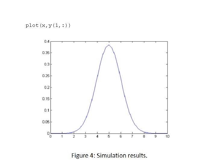
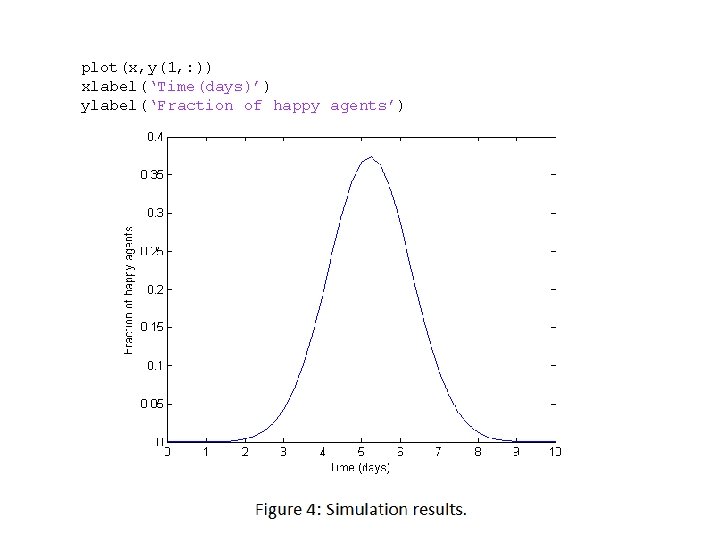
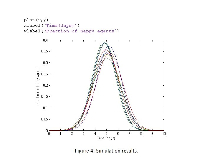
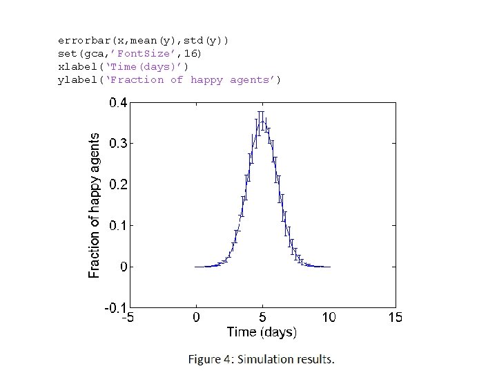
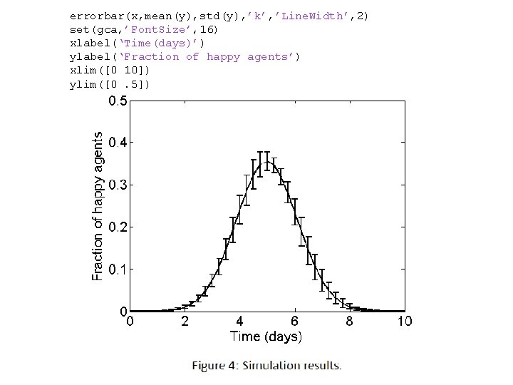
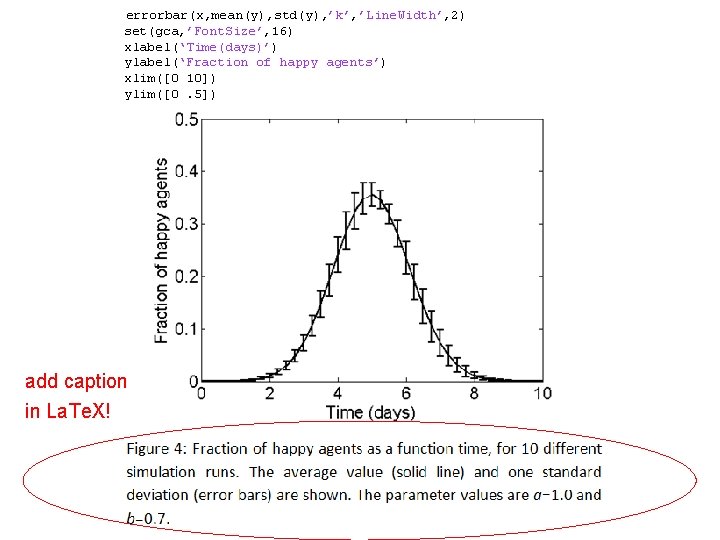
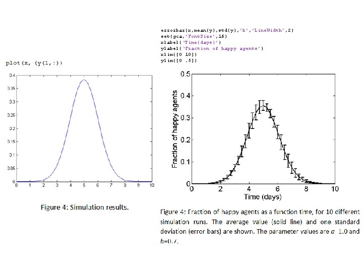
Example § As an example: Let us say that we have a project about simulating happiness of agents. § We have the result of 10 different simulation runs in y, and the corresponding time vector in x. § x = t 0: dt: t 1; y = [happiness values from simulation 1; happiness values from simulation 2; . . . happiness values from simulation 10]; 2011 -05 -02 K. Donnay & S. Balietti / kdonnay@ethz. ch sbalietti@ethz. ch 16

plot(x, y(1, : )) 2011 -05 -02 K. Donnay & S. Balietti / kdonnay@ethz. ch sbalietti@ethz. ch 17

plot(x, y(1, : )) xlabel(‘Time(days)’) ylabel(‘Fraction of happy agents’) 2011 -05 -02 K. Donnay & S. Balietti / kdonnay@ethz. ch sbalietti@ethz. ch 18

plot(x, y) xlabel(‘Time(days)’) ylabel(‘Fraction of happy agents’) 2011 -05 -02 K. Donnay & S. Balietti / kdonnay@ethz. ch sbalietti@ethz. ch 19

plot(x, y) set(gca, ’Font. Size’, 16) xlabel(‘Time(days)’) ylabel(‘Fraction of happy agents’) 2011 -05 -02 K. Donnay & S. Balietti / kdonnay@ethz. ch sbalietti@ethz. ch 20

errorbar(x, mean(y), std(y)) set(gca, ’Font. Size’, 16) xlabel(‘Time(days)’) ylabel(‘Fraction of happy agents’) 2011 -05 -02 K. Donnay & S. Balietti / kdonnay@ethz. ch sbalietti@ethz. ch 21

errorbar(x, mean(y), std(y), ’k’, ’Line. Width’, 2) set(gca, ’Font. Size’, 16) xlabel(‘Time(days)’) ylabel(‘Fraction of happy agents’) xlim([0 10]) ylim([0. 5]) 2011 -05 -02 K. Donnay & S. Balietti / kdonnay@ethz. ch sbalietti@ethz. ch 22

errorbar(x, mean(y), std(y), ’k’, ’Line. Width’, 2) set(gca, ’Font. Size’, 16) xlabel(‘Time(days)’) ylabel(‘Fraction of happy agents’) xlim([0 10]) ylim([0. 5]) add caption in La. Te. X! 2011 -05 -02 K. Donnay & S. Balietti / kdonnay@ethz. ch sbalietti@ethz. ch 23

errorbar(x, mean(y), std(y), ’k’, ’Line. Width’, 2) set(gca, ’Font. Size’, 16) xlabel(‘Time(days)’) ylabel(‘Fraction of happy agents’) xlim([0 10]) ylim([0. 5]) 2011 -05 -02 K. Donnay & S. Balietti / kdonnay@ethz. ch sbalietti@ethz. ch 24

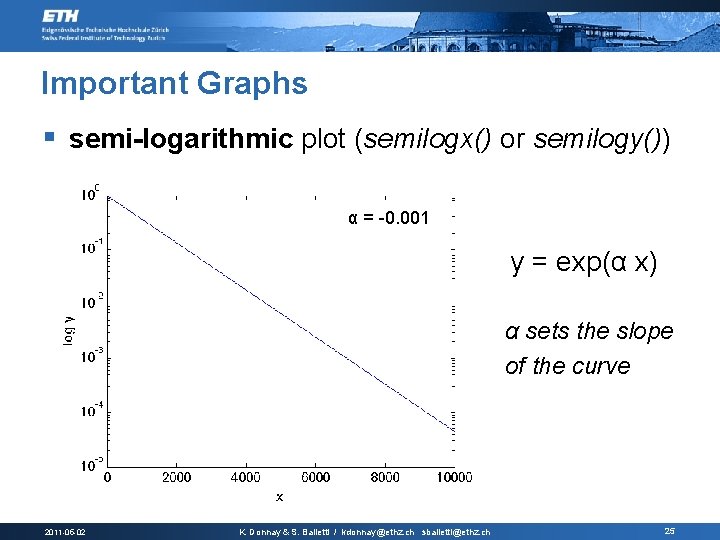
Important Graphs § semi-logarithmic plot (semilogx() or semilogy()) α = -0. 001 y = exp(α x) α sets the slope of the curve 2011 -05 -02 K. Donnay & S. Balietti / kdonnay@ethz. ch sbalietti@ethz. ch 25

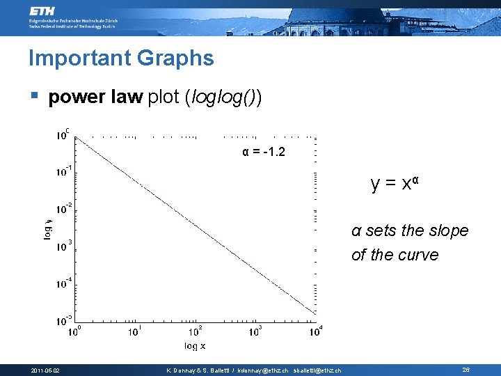
Important Graphs § power law plot (loglog()) α = -1. 2 y = xα α sets the slope of the curve 2011 -05 -02 K. Donnay & S. Balietti / kdonnay@ethz. ch sbalietti@ethz. ch 26

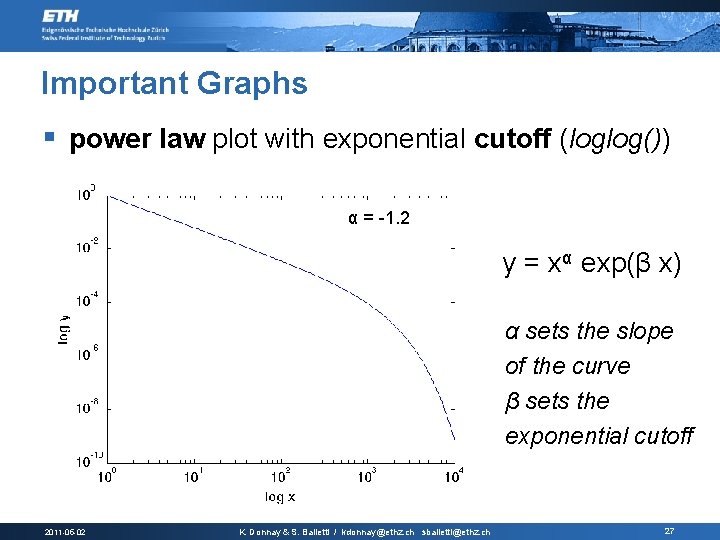
Important Graphs § power law plot with exponential cutoff (loglog()) α = -1. 2 y = xα exp(β x) α sets the slope of the curve β sets the exponential cutoff 2011 -05 -02 K. Donnay & S. Balietti / kdonnay@ethz. ch sbalietti@ethz. ch 27

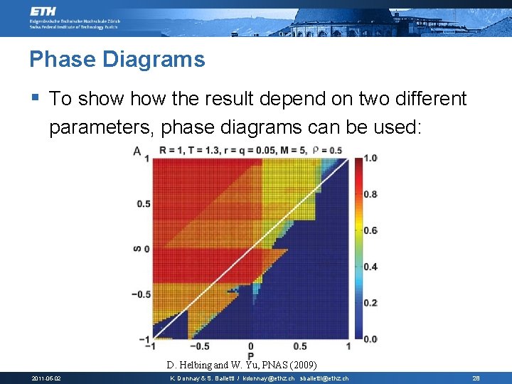
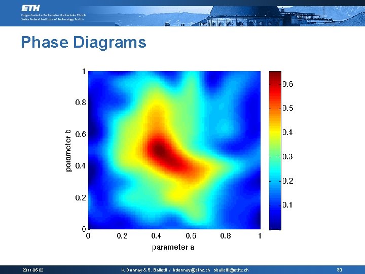
Phase Diagrams § To show the result depend on two different parameters, phase diagrams can be used: D. Helbing and W. Yu, PNAS (2009) 2011 -05 -02 K. Donnay & S. Balietti / kdonnay@ethz. ch sbalietti@ethz. ch 28

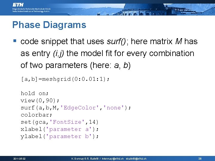
Phase Diagrams § code snippet that uses surf(); here matrix M has as entry (i, j) the model fit for every combination of two parameters (here: a, b) [a, b]=meshgrid(0: 0. 01: 1); hold on; view(0, 90); surf(a, b, M, 'Edge. Color', 'none'); colorbar; set(gca, 'Font. Size', 14) xlabel('parameter a'); ylabel('parameter b'); 2011 -05 -02 K. Donnay & S. Balietti / kdonnay@ethz. ch sbalietti@ethz. ch 29

Phase Diagrams 2011 -05 -02 K. Donnay & S. Balietti / kdonnay@ethz. ch sbalietti@ethz. ch 30

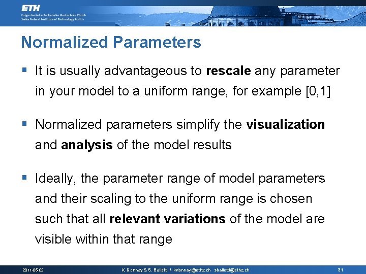
Normalized Parameters § It is usually advantageous to rescale any parameter in your model to a uniform range, for example [0, 1] § Normalized parameters simplify the visualization and analysis of the model results § Ideally, the parameter range of model parameters and their scaling to the uniform range is chosen such that all relevant variations of the model are visible within that range 2011 -05 -02 K. Donnay & S. Balietti / kdonnay@ethz. ch sbalietti@ethz. ch 31

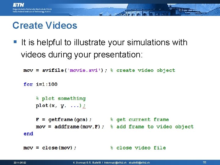
Create Videos § It is helpful to illustrate your simulations with videos during your presentation: 2011 -05 -02 K. Donnay & S. Balietti / kdonnay@ethz. ch sbalietti@ethz. ch 32

Project Report § Have a look at last year’s projects to make sure that you don’t repeat the same results! § Use the report template. § Try to explain your results well, as well as explaining your motivation behind the project. § Include your MATLAB code in the appendix § If you have any problems or concerns with your projects, we are here to help you! 2011 -05 -02 K. Donnay & S. Balietti / kdonnay@ethz. ch sbalietti@ethz. ch 33

Project Report § There a number of things that will certainly negatively affect your grade: § no clearly stated research question § no conclusion regarding the work you have completed and how it relates to your research question § graphs which have no legend, axis labels or caption, are not properly readable or the labels are too small § no references to the literature to validate and back-up your statements/model etc. § submitting you report late or incomplete 2011 -05 -02 K. Donnay & S. Balietti / kdonnay@ethz. ch sbalietti@ethz. ch 34

Project Report § References are very important: § cite the sources you are using § be aware that plagiarism is taken very seriously at ETH, if you are unsure how to cite properly follow ETH’s plagiarism guidelines § we accept both natural science and social science citation conventions but please use them consistently § it is important that your references are correct and correctly formatted! 2011 -05 -02 K. Donnay & S. Balietti / kdonnay@ethz. ch sbalietti@ethz. ch 35

Project Report § Documentation of your code is important § You can, for example, use the following tool to automatically generate html files from comments in your code http: //www. artefact. tk/software/matlab/m 2 html/ § Please also pay attention to the MATLAB code style guidelines provided here to guarantee that your code is flawless and easy to understand 2011 -05 -02 K. Donnay & S. Balietti / kdonnay@ethz. ch sbalietti@ethz. ch 36

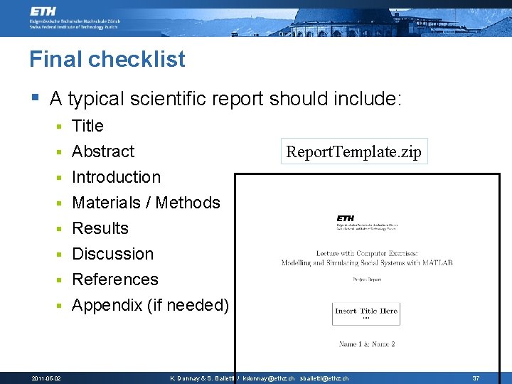
Final checklist § A typical scientific report should include: § § § § 2011 -05 -02 Title Abstract Introduction Materials / Methods Results Discussion References Appendix (if needed) Report. Template. zip K. Donnay & S. Balietti / kdonnay@ethz. ch sbalietti@ethz. ch 37

References § MATLAB documentation on plotting § MATLAB code style guidelines § Tool to convert comments to html files § J. -L. Dumont. “Trees, maps and theorems”. Principiae (2009). § Russey, Ebel, Bliefert. “How to Write a Successful Science Thesis”. Wiley (2006). § R. Murray. “How to Write a Thesis”. Open University Press (2006) 2011 -05 -02 K. Donnay & S. Balietti / kdonnay@ethz. ch sbalietti@ethz. ch 38