4 4 Laws Of Logarithms Laws of Logarithms

4. 4 Laws Of Logarithms

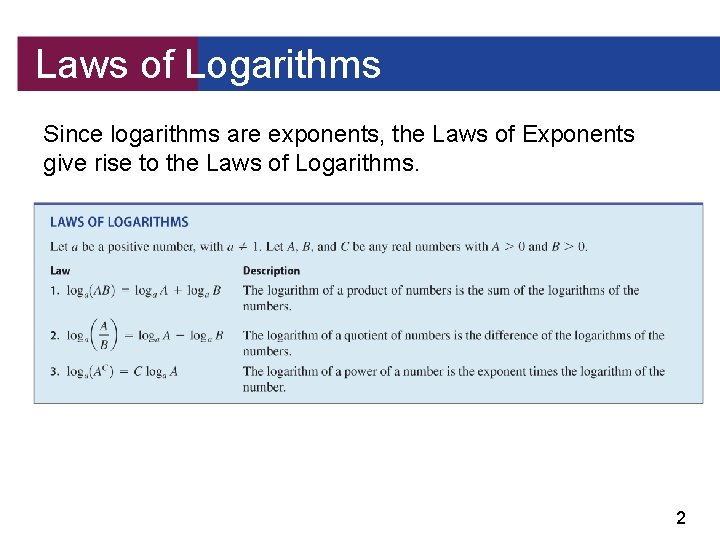
Laws of Logarithms Since logarithms are exponents, the Laws of Exponents give rise to the Laws of Logarithms. 2

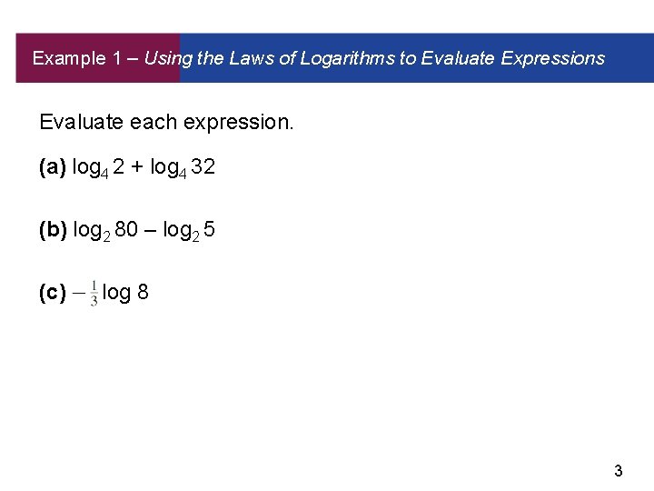
Example 1 – Using the Laws of Logarithms to Evaluate Expressions Evaluate each expression. (a) log 4 2 + log 4 32 (b) log 2 80 – log 2 5 (c) log 8 3

Expanding and Combining Logarithmic Expressions The Laws of Logarithms allow us to write the logarithm of a product or a quotient as the sum or difference of logarithms. This process, called expanding a logarithmic expression, is illustrated in the next example. 4

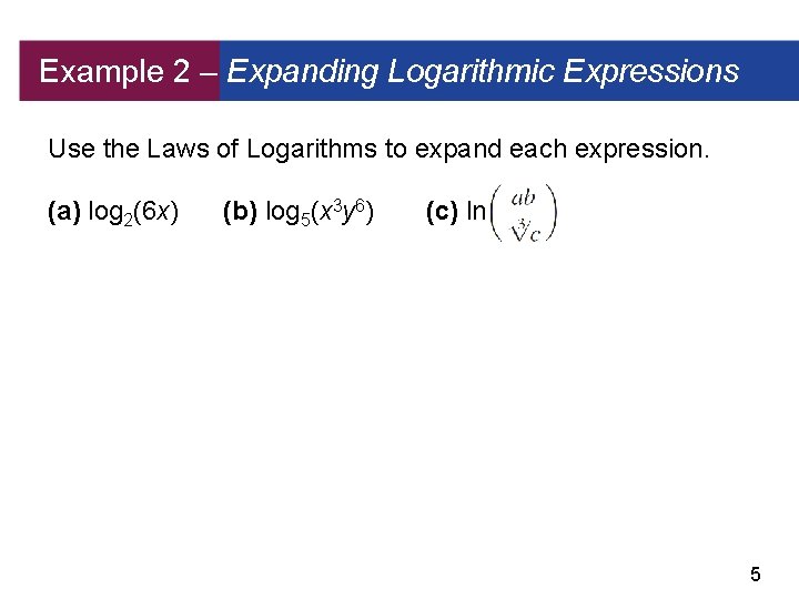
Example 2 – Expanding Logarithmic Expressions Use the Laws of Logarithms to expand each expression. (a) log 2(6 x) (b) log 5(x 3 y 6) (c) ln 5

Expanding and Combining Logarithmic Expressions The Laws of Logarithms also allow us to reverse the process of expanding that was done in Example 2. That is, we can write sums and differences of logarithms as a single logarithm. This process, called combining logarithmic expressions, is illustrated in the next example. 6

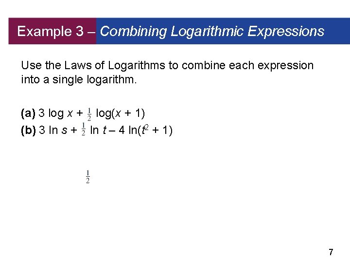
Example 3 – Combining Logarithmic Expressions Use the Laws of Logarithms to combine each expression into a single logarithm. (a) 3 log x + log(x + 1) (b) 3 ln s + ln t – 4 ln(t 2 + 1) 7

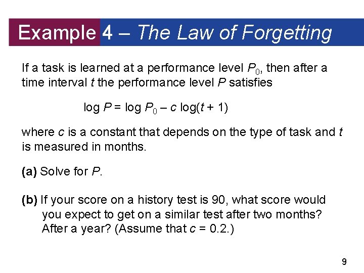
Expanding and Combining Logarithmic Expressions Logarithmic functions are used to model a variety of situations involving human behavior. One such behavior is how quickly we forget things we have learned. For example, if you learn algebra at a certain performance level (say, 90% on a test) and then don’t use algebra for a while, how much will you retain after a week, a month, or a year? Hermann Ebbinghaus (1850– 1909) studied this phenomenon and formulated the law described in the next example. 8

Example 4 – The Law of Forgetting If a task is learned at a performance level P 0, then after a time interval t the performance level P satisfies log P = log P 0 – c log(t + 1) where c is a constant that depends on the type of task and t is measured in months. (a) Solve for P. (b) If your score on a history test is 90, what score would you expect to get on a similar test after two months? After a year? (Assume that c = 0. 2. ) 9

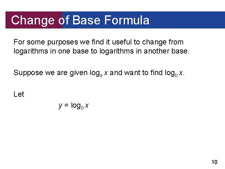
Change of Base Formula For some purposes we find it useful to change from logarithms in one base to logarithms in another base. Suppose we are given loga x and want to find logb x. Let y = logb x 10

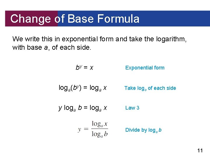
Change of Base Formula We write this in exponential form and take the logarithm, with base a, of each side. by = x Exponential form loga (by) = loga x Take loga of each side y loga b = loga x Law 3 Divide by loga b 11

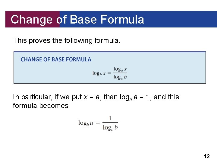
Change of Base Formula This proves the following formula. In particular, if we put x = a, then loga a = 1, and this formula becomes 12

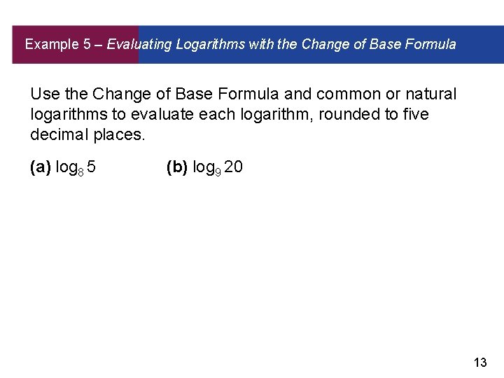
Example 5 – Evaluating Logarithms with the Change of Base Formula Use the Change of Base Formula and common or natural logarithms to evaluate each logarithm, rounded to five decimal places. (a) log 8 5 (b) log 9 20 13

4. 5 Exponential and Logarithmic Equations 14

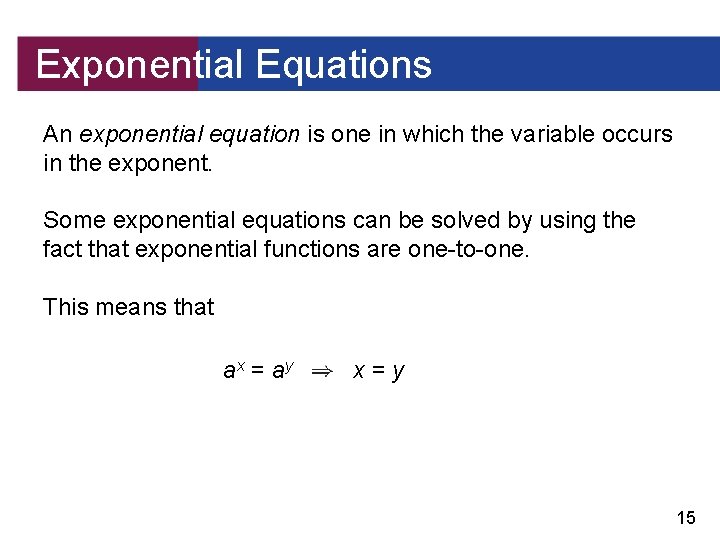
Exponential Equations An exponential equation is one in which the variable occurs in the exponent. Some exponential equations can be solved by using the fact that exponential functions are one-to-one. This means that ax = ay x=y 15

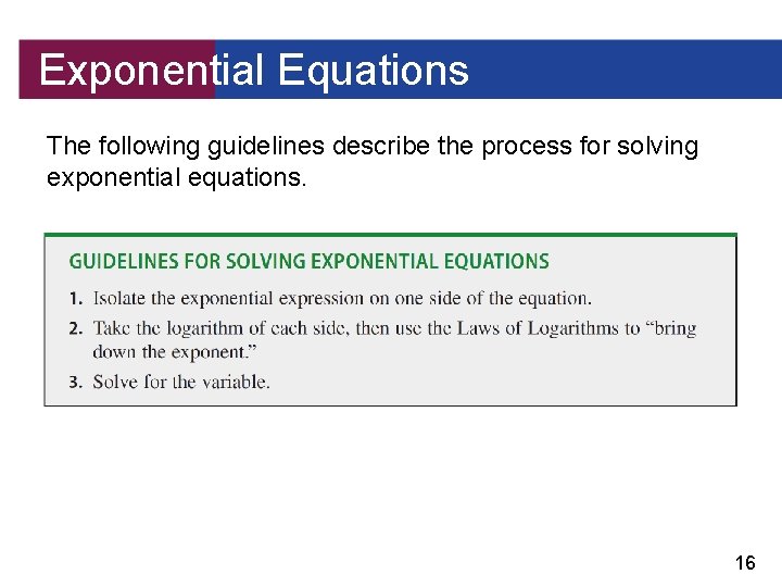
Exponential Equations The following guidelines describe the process for solving exponential equations. 16

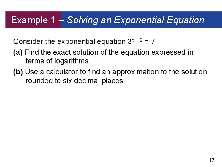
Example 1 – Solving an Exponential Equation Consider the exponential equation 3 x + 2 = 7. (a) Find the exact solution of the equation expressed in terms of logarithms. (b) Use a calculator to find an approximation to the solution rounded to six decimal places. 17

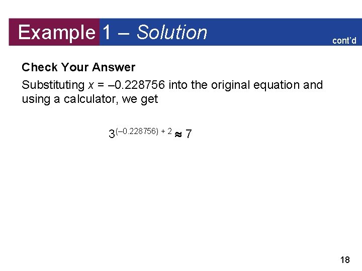
Example 1 – Solution cont’d Check Your Answer Substituting x = – 0. 228756 into the original equation and using a calculator, we get 3(– 0. 228756) + 2 7 18

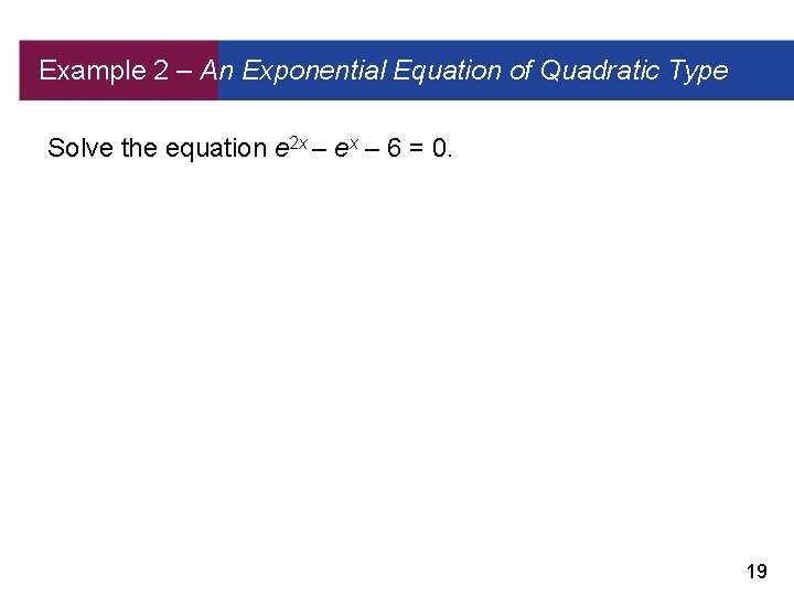
Example 2 – An Exponential Equation of Quadratic Type Solve the equation e 2 x – ex – 6 = 0. 19

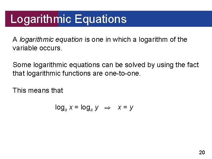
Logarithmic Equations A logarithmic equation is one in which a logarithm of the variable occurs. Some logarithmic equations can be solved by using the fact that logarithmic functions are one-to-one. This means that loga x = loga y x=y 20

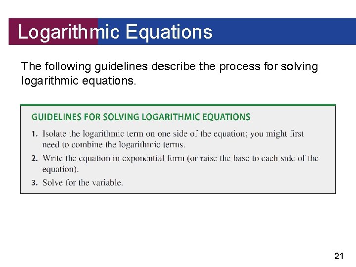
Logarithmic Equations The following guidelines describe the process for solving logarithmic equations. 21

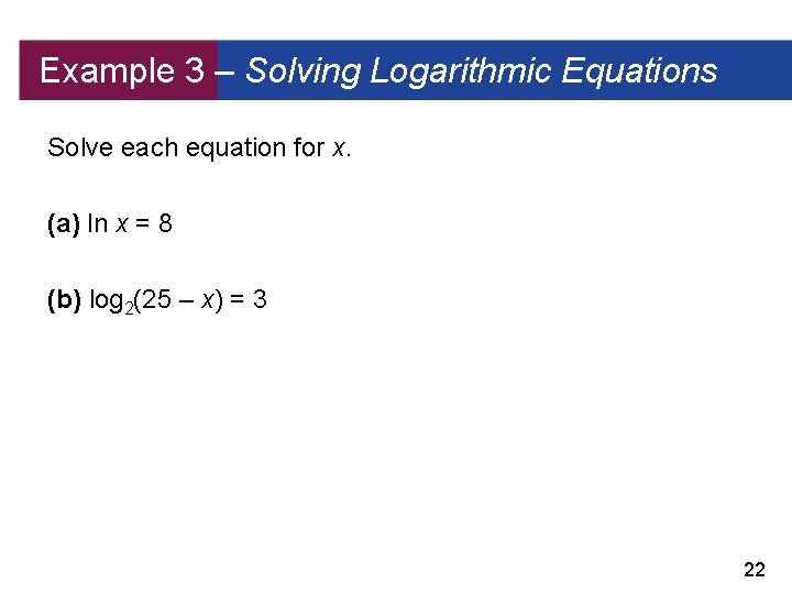
Example 3 – Solving Logarithmic Equations Solve each equation for x. (a) ln x = 8 (b) log 2(25 – x) = 3 22

Logarithmic Equations Logarithmic equations are used in determining the amount of light that reaches various depths in a lake. (This information helps biologists to determine the types of life a lake can support. ) As light passes through water (or other transparent materials such as glass or plastic), some of the light is absorbed. It’s easy to see that the murkier the water, the more light is absorbed. The exact relationship between light absorption and the distance light travels in a material is described in the next example. 23

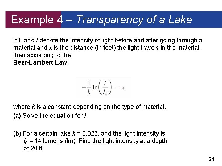
Example 4 – Transparency of a Lake If I 0 and I denote the intensity of light before and after going through a material and x is the distance (in feet) the light travels in the material, then according to the Beer-Lambert Law, where k is a constant depending on the type of material. (a) Solve the equation for I. (b) For a certain lake k = 0. 025, and the light intensity is I 0 = 14 lumens (lm). Find the light intensity at a depth of 20 ft. 24

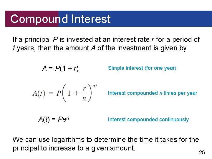
Compound Interest If a principal P is invested at an interest rate r for a period of t years, then the amount A of the investment is given by A = P(1 + r) Simple interest (for one year) Interest compounded n times per year A(t) = Pert Interest compounded continuously We can use logarithms to determine the time it takes for the principal to increase to a given amount. 25

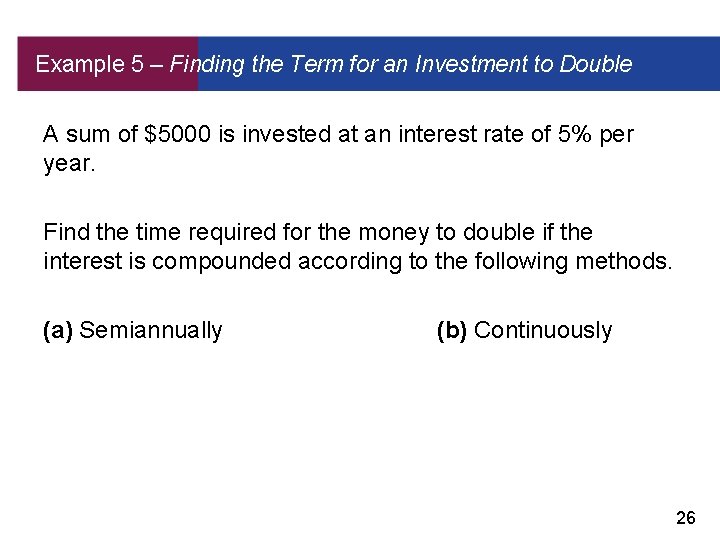
Example 5 – Finding the Term for an Investment to Double A sum of $5000 is invested at an interest rate of 5% per year. Find the time required for the money to double if the interest is compounded according to the following methods. (a) Semiannually (b) Continuously 26

4. 6 Modeling with Exponential Functions 27

Modeling with Exponential Functions Many processes that occur in nature, such as population growth, radioactive decay, heat diffusion, and numerous others, can be modeled by using exponential functions. In this section we study exponential models. 28

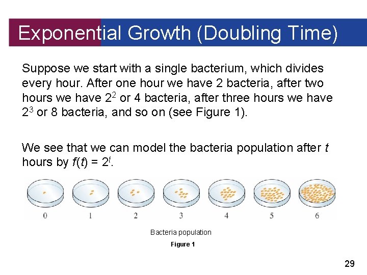
Exponential Growth (Doubling Time) Suppose we start with a single bacterium, which divides every hour. After one hour we have 2 bacteria, after two hours we have 22 or 4 bacteria, after three hours we have 23 or 8 bacteria, and so on (see Figure 1). We see that we can model the bacteria population after t hours by f (t) = 2 t. Bacteria population Figure 1 29

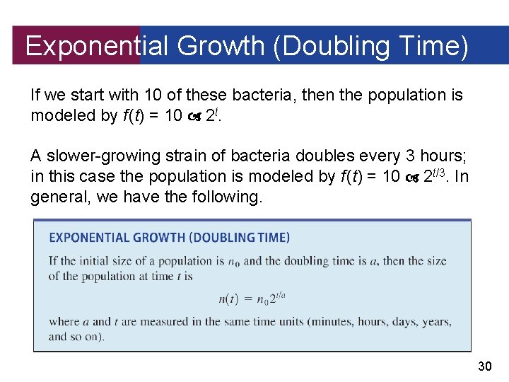
Exponential Growth (Doubling Time) If we start with 10 of these bacteria, then the population is modeled by f (t) = 10 2 t. A slower-growing strain of bacteria doubles every 3 hours; in this case the population is modeled by f (t) = 10 2 t/3. In general, we have the following. 30

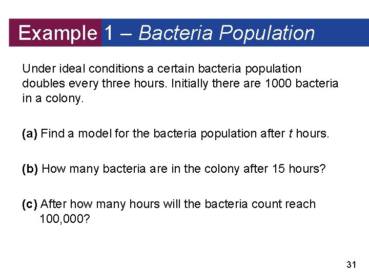
Example 1 – Bacteria Population Under ideal conditions a certain bacteria population doubles every three hours. Initially there are 1000 bacteria in a colony. (a) Find a model for the bacteria population after t hours. (b) How many bacteria are in the colony after 15 hours? (c) After how many hours will the bacteria count reach 100, 000? 31

Exponential Growth (Relative Growth Rate) 32

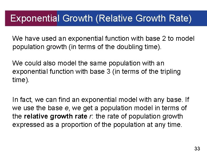
Exponential Growth (Relative Growth Rate) We have used an exponential function with base 2 to model population growth (in terms of the doubling time). We could also model the same population with an exponential function with base 3 (in terms of the tripling time). In fact, we can find an exponential model with any base. If we use the base e, we get a population model in terms of the relative growth rate r: the rate of population growth expressed as a proportion of the population at any time. 33

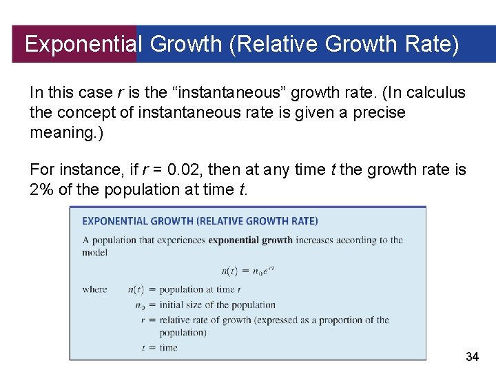
Exponential Growth (Relative Growth Rate) In this case r is the “instantaneous” growth rate. (In calculus the concept of instantaneous rate is given a precise meaning. ) For instance, if r = 0. 02, then at any time t the growth rate is 2% of the population at time t. 34

Exponential Growth (Relative Growth Rate) Notice that the formula for population growth is the same as that for continuously compounded interest. In fact, the same principle is at work in both cases: The growth of a population (or an investment) per time period is proportional to the size of the population (or the amount of the investment). A population of 1, 000 will increase more in one year than a population of 1000; in exactly the same way, an investment of $1, 000 will increase more in one year than an investment of $1000. In the next example we assume that the populations grow exponentially. 35

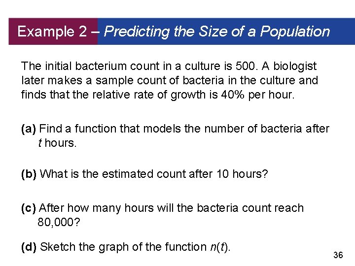
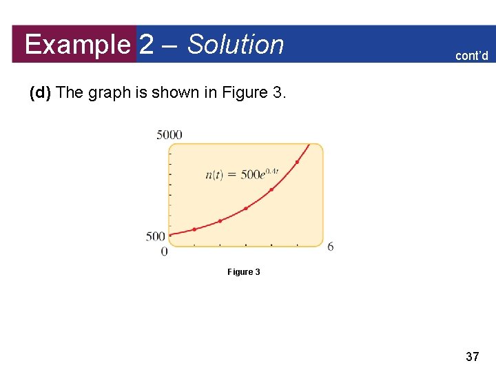
Example 2 – Predicting the Size of a Population The initial bacterium count in a culture is 500. A biologist later makes a sample count of bacteria in the culture and finds that the relative rate of growth is 40% per hour. (a) Find a function that models the number of bacteria after t hours. (b) What is the estimated count after 10 hours? (c) After how many hours will the bacteria count reach 80, 000? (d) Sketch the graph of the function n(t). 36

Example 2 – Solution cont’d (d) The graph is shown in Figure 3 37

Radioactive Decay Radioactive substances decay by spontaneously emitting radiation. The rate of decay is proportional to the mass of the substance. This is analogous to population growth except that the mass decreases. Physicists express the rate of decay in terms of half-life, the time it takes for a sample of the substance to decay to half its original mass. For example, the half-life of radium-226 is 1600 years, so a 100 -g sample decays to 50 g (or 100 g) in 1600 years, then to 25 g (or 100 g) in 3200 years, and so on. 38

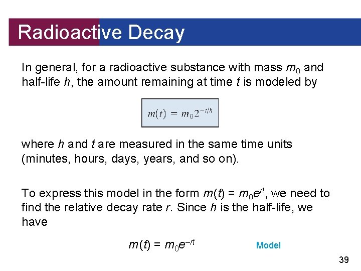
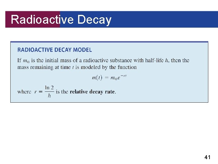
Radioactive Decay In general, for a radioactive substance with mass m 0 and half-life h, the amount remaining at time t is modeled by where h and t are measured in the same time units (minutes, hours, days, years, and so on). To express this model in the form m (t) = m 0 ert, we need to find the relative decay rate r. Since h is the half-life, we have m (t) = m 0 e–rt Model 39

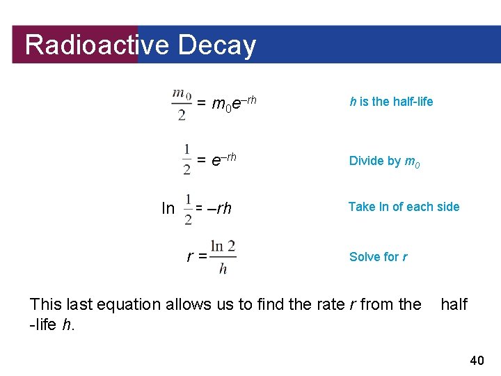
Radioactive Decay ln = m 0 e–rh h is the half-life = e–rh Divide by m 0 = –rh r= Take ln of each side Solve for r This last equation allows us to find the rate r from the -life h. half 40

Radioactive Decay 41

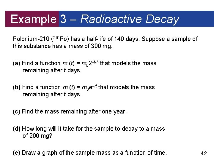
Example 3 – Radioactive Decay Polonium-210 (210 Po) has a half-life of 140 days. Suppose a sample of this substance has a mass of 300 mg. (a) Find a function m (t) = m 02–t/h that models the mass remaining after t days. (b) Find a function m (t) = m 0 e–rt that models the mass remaining after t days. (c) Find the mass remaining after one year. (d) How long will it take for the sample to decay to a mass of 200 mg? (e) Draw a graph of the sample mass as a function of time. 42

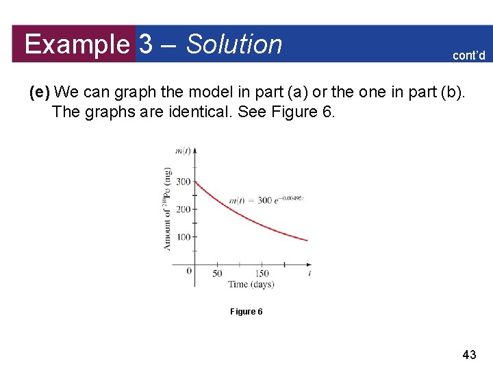
Example 3 – Solution cont’d (e) We can graph the model in part (a) or the one in part (b). The graphs are identical. See Figure 6 43

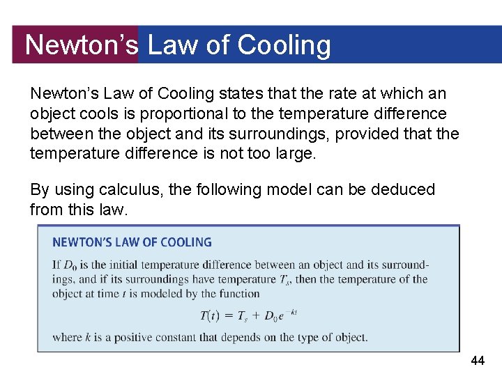
Newton’s Law of Cooling states that the rate at which an object cools is proportional to the temperature difference between the object and its surroundings, provided that the temperature difference is not too large. By using calculus, the following model can be deduced from this law. 44

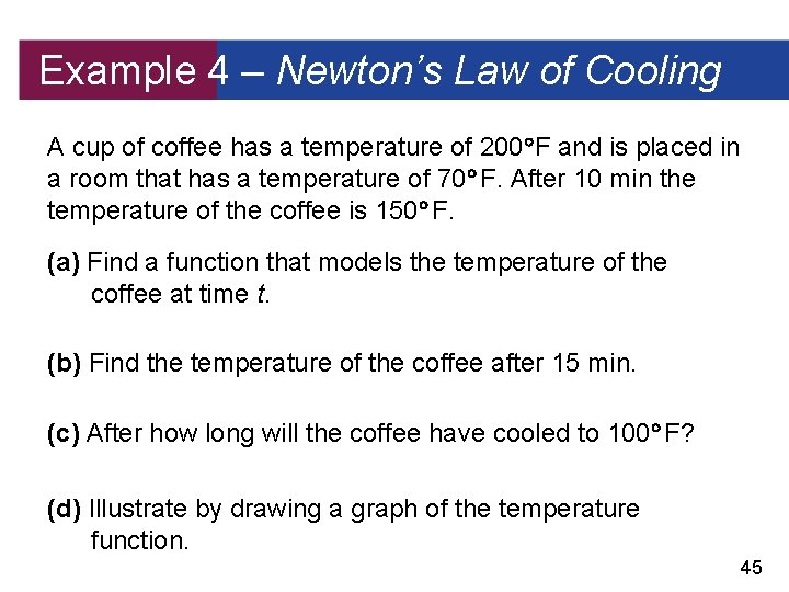
Example 4 – Newton’s Law of Cooling A cup of coffee has a temperature of 200 F and is placed in a room that has a temperature of 70 F. After 10 min the temperature of the coffee is 150 F. (a) Find a function that models the temperature of the coffee at time t. (b) Find the temperature of the coffee after 15 min. (c) After how long will the coffee have cooled to 100 F? (d) Illustrate by drawing a graph of the temperature function. 45

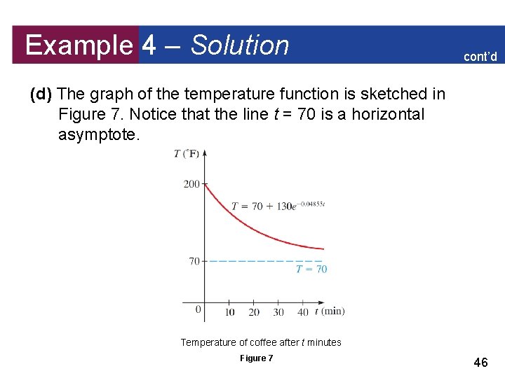
Example 4 – Solution cont’d (d) The graph of the temperature function is sketched in Figure 7. Notice that the line t = 70 is a horizontal asymptote. Temperature of coffee after t minutes Figure 7 46