3 2 1 BPSK BPSK 3 2 Data
![3. 2. 1 BPSK 변조방식의 기본 구성 BPSK] [3. 2 § Data generator Pulse](http://slidetodoc.com/presentation_image_h2/fbcbb5a9ed18d19fefbc7ab28ae43ab8/image-3.jpg "3. 2. 1 BPSK 변조방식의 기본 구성 BPSK] [3. 2 § Data generator Pulse")
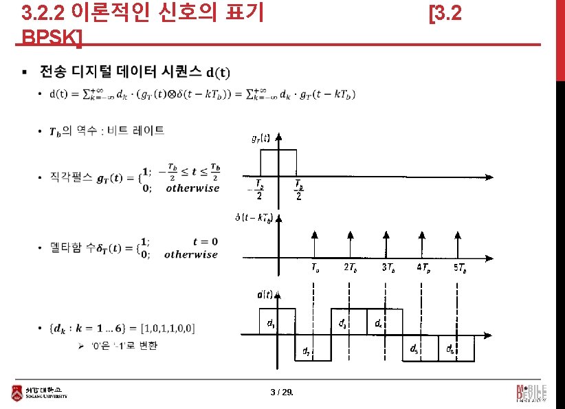
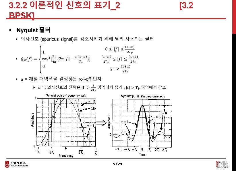
3. 2. 1 BPSK 변조방식의 기본 구성 BPSK] [3. 2 § Data generator Pulse shaping filter Data X D/A BPF DPSH (Digital Signal Processing Hardware) Bandpass filter X BPF A/D Pulse shaping filter Pulse compensator Decision circuit - 필터링 (심볼간섭 제거) - 필터링 된 신호에서 동기화 지점이 선택 - 동기화 지점에서 신호레벨 > 0 , 수신된 신호 데이터 : 1 - 동기화 지점에서 신호레벨 < 0 , 수신된 신호 데이터 : 0 2 / 29.
![3. 2. 3 컴퓨터 시뮬레이션 프로그램_1_1 BPSK] § [3. 2 이론적인 관계 § 공통변수](http://slidetodoc.com/presentation_image_h2/fbcbb5a9ed18d19fefbc7ab28ae43ab8/image-13.jpg "3. 2. 3 컴퓨터 시뮬레이션 프로그램_1_1 BPSK] § [3. 2 이론적인 관계 § 공통변수")
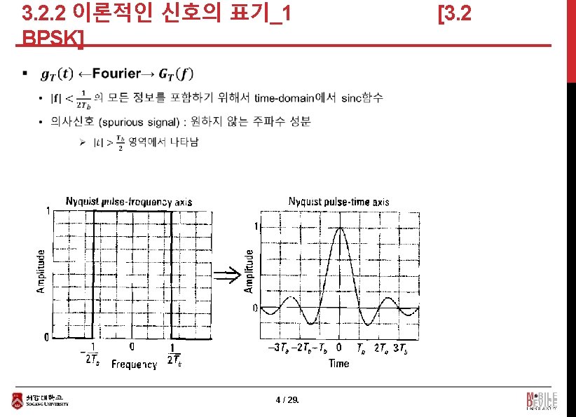
3. 2. 3 컴퓨터 시뮬레이션 프로그램_1_1 BPSK] § [3. 2 이론적인 관계 § 공통변수 설정 → Root Nyquist 필터의 필터계수 설정 → Data generation → BPSK Modulation → Attenuation Calculation → Add white Gaussian Noise (AWGN) → BPSK Demodulation → Bit Error Rate (BER) 12 / 29.
![3. 2. 3 컴퓨터 시뮬레이션 프로그램_1_2 BPSK] § 공통변수 설정 § Root Nyquist 필터의](http://slidetodoc.com/presentation_image_h2/fbcbb5a9ed18d19fefbc7ab28ae43ab8/image-14.jpg "3. 2. 3 컴퓨터 시뮬레이션 프로그램_1_2 BPSK] § 공통변수 설정 § Root Nyquist 필터의")
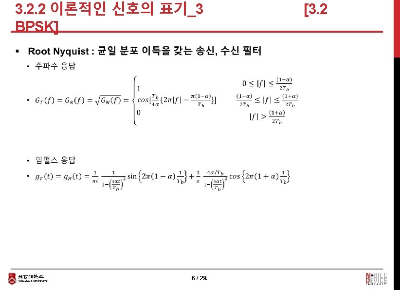
3. 2. 3 컴퓨터 시뮬레이션 프로그램_1_2 BPSK] § 공통변수 설정 § Root Nyquist 필터의 필터계수 설정 (hrollfcoef. m) • function [xh]=hrollfcoef(irfn, ipoint, sr, alfs, ncc) Ø irfn = Number of symbols to use filtering Ø ipoint = number of samples in one symbol Ø sr = symbol rate Ø alfs = Rolloff coefficiense Ø ncc = (1 : transmitting filter) , (0 : receiving filter) 13 / 29. [3. 2
![3. 2. 3 컴퓨터 시뮬레이션 프로그램_1_6 BPSK] • data 5=conv(data 4, xh 2); %](http://slidetodoc.com/presentation_image_h2/fbcbb5a9ed18d19fefbc7ab28ae43ab8/image-18.jpg "3. 2. 3 컴퓨터 시뮬레이션 프로그램_1_6 BPSK] • data 5=conv(data 4, xh 2); %")
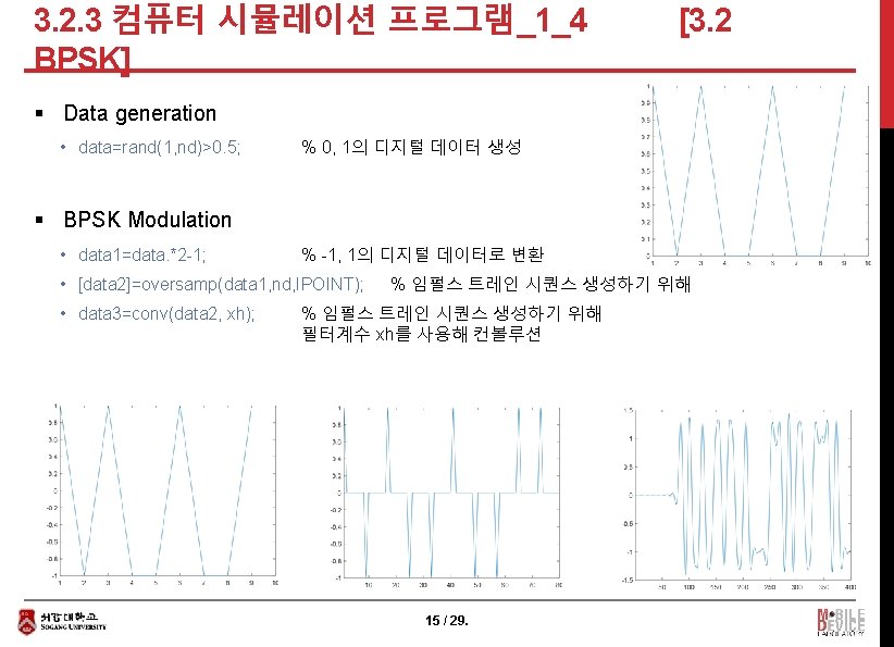
3. 2. 3 컴퓨터 시뮬레이션 프로그램_1_6 BPSK] • data 5=conv(data 4, xh 2); % 필터계수 xh 2를 갖는 Root Nyquist로 필터링 § conv 사용 → length(xh) 의 time delay = (irfn*IPOINT)/2 • 2번의 conv 사용으로 irfn*IPOINT 의 time delay 생김 • time delay를 복원하기 위해 resample • samp 1=irfn*IPOINT+1; % 재샘플의 시작지점 • data 6=data 5(samp 1: 8: 8*nd+samp 1 -1); % 재샘플링된 신호 data 6 • % 송신신호가 복원 17 / 29. [3. 2
![3. 2. 3 컴퓨터 시뮬레이션 프로그램_1_8 BPSK] § Bit Error Rate (BER) • noe](http://slidetodoc.com/presentation_image_h2/fbcbb5a9ed18d19fefbc7ab28ae43ab8/image-20.jpg "3. 2. 3 컴퓨터 시뮬레이션 프로그램_1_8 BPSK] § Bit Error Rate (BER) • noe")
3. 2. 3 컴퓨터 시뮬레이션 프로그램_1_8 BPSK] § Bit Error Rate (BER) • noe 2=sum(abs(data-demodata)); • nod 2=length(data); % bit error의 수 % data의 길이 • noe=noe+noe 2; • nod=nod+nod 2; • ber=noe/nod; % BER 19 / 29. [3. 2
![3. 2. 3 컴퓨터 시뮬레이션 프로그램_2_1 BPSK] [3. 2 § BPSK_fading : 레일리 페이딩](http://slidetodoc.com/presentation_image_h2/fbcbb5a9ed18d19fefbc7ab28ae43ab8/image-21.jpg "3. 2. 3 컴퓨터 시뮬레이션 프로그램_2_1 BPSK] [3. 2 § BPSK_fading : 레일리 페이딩")
3. 2. 3 컴퓨터 시뮬레이션 프로그램_2_1 BPSK] [3. 2 § BPSK_fading : 레일리 페이딩 환경에서의 시뮬레이션 § 공통변수 설정 → Nyquist 필터의 필터계수 설정 → Fading initialization → Data generation → BPSK Modulation → Attenuation Calculation → Fading channel → Add white Gaussian Noise (AWGN) → BPSK Demodulation → Bit Error Rate (BER) § Fading initialization • tstp=1/sr/IPOINT; % Time resolution • itau=[0]; % arrival time for each multipath normalized by tstp • dlvl=[0]; % Mean power for each multipath normalized by direct wave • n 0=[6]; % Number of waves to generate fading for each multipath • th 1=[0. 0]; % Initial Phase of delayed wave • itnd 0=nd*IPOINT*100; % Number of fading counter to skip • itnd 1=[1000]; % Initial value of fading counter • now 1=1; % Number of directwave + Number of delayed wave • fd=160; % Maximum Doppler frequency [Hz] • flat=1; % (1→flat (only amplitude is fluctuated) (0→normal phase and amplitude are fluctuated) 20 / 29.
![3. 2. 3 컴퓨터 시뮬레이션 프로그램_2_2 BPSK] [3. 2 § Fading channel • [ifade,](http://slidetodoc.com/presentation_image_h2/fbcbb5a9ed18d19fefbc7ab28ae43ab8/image-22.jpg "3. 2. 3 컴퓨터 시뮬레이션 프로그램_2_2 BPSK] [3. 2 § Fading channel • [ifade,")
3. 2. 3 컴퓨터 시뮬레이션 프로그램_2_2 BPSK] [3. 2 § Fading channel • [ifade, qfade] % generated data are fed into a fading simulator =sefade(data 3, zeros(1, length(data 3)), itau, dlvl, th 1, n 0, itnd 1, now 1, length(data 3), tstp, fd, flat); • itnd 1=itnd 1+itnd 0; % update fading counter § Add white Gaussian Noise (AWGN) • inoise=randn(1, length(ifade)). *attn; • data 4=ifade+inoise; § BPSK vs. BPSK_fading 21 / 29.
![3. 3. 3 컴퓨터 시뮬레이션_1 [3. 3 QPSK] § Ich 와 Qch의 두 시뮬레이션의](http://slidetodoc.com/presentation_image_h2/fbcbb5a9ed18d19fefbc7ab28ae43ab8/image-26.jpg "3. 3. 3 컴퓨터 시뮬레이션_1 [3. 3 QPSK] § Ich 와 Qch의 두 시뮬레이션의")
3. 3. 3 컴퓨터 시뮬레이션_1 [3. 3 QPSK] § Ich 와 Qch의 두 시뮬레이션의 흐름이 존재 • 두 시뮬레이션은 독립적 • BPSK의 시뮬레이션과 동일 § 공통변수 설정 → Root Nyquist 필터의 필터계수 설정 → Data generation → QPSK Modulation → Attenuation Calculation → Add white Gaussian Noise (AWGN) → QPSK Demodulation → Bit Error Rate (BER) 25 / 29.
![3. 3. 3 컴퓨터 시뮬레이션_2 [3. 3 QPSK] § 공통변수 설정→Root Nyquist 필터의 필터계수](http://slidetodoc.com/presentation_image_h2/fbcbb5a9ed18d19fefbc7ab28ae43ab8/image-27.jpg "3. 3. 3 컴퓨터 시뮬레이션_2 [3. 3 QPSK] § 공통변수 설정→Root Nyquist 필터의 필터계수")
3. 3. 3 컴퓨터 시뮬레이션_2 [3. 3 QPSK] § 공통변수 설정→Root Nyquist 필터의 필터계수 설정 § Data generation • data 1=rand(1, nd*ml)>0. 5; % ml=2 § QPSK Modulation • [ich, qch]=qpskmod(data 1, 1, nd, ml); 26 / 29.
![3. 3. 3 컴퓨터 시뮬레이션_3 [3. 3 QPSK] § Attenuation Calculation → Add white](http://slidetodoc.com/presentation_image_h2/fbcbb5a9ed18d19fefbc7ab28ae43ab8/image-28.jpg "3. 3. 3 컴퓨터 시뮬레이션_3 [3. 3 QPSK] § Attenuation Calculation → Add white")
3. 3. 3 컴퓨터 시뮬레이션_3 [3. 3 QPSK] § Attenuation Calculation → Add white Gaussian Noise (AWGN) § QPSK Demodulation • [demodata]=qpskdemod(ich 5, qch 5, 1, nd, ml); Output data 27 / 29.
![3. 3. 3 컴퓨터 시뮬레이션_4 [3. 3 QPSK] data generation AWGN QPSK modulation (ich,](http://slidetodoc.com/presentation_image_h2/fbcbb5a9ed18d19fefbc7ab28ae43ab8/image-29.jpg "3. 3. 3 컴퓨터 시뮬레이션_4 [3. 3 QPSK] data generation AWGN QPSK modulation (ich,")
3. 3. 3 컴퓨터 시뮬레이션_4 [3. 3 QPSK] data generation AWGN QPSK modulation (ich, qch) over sampling 송신기 필터와 convolution 수신기 필터와 convolution resampling QPSK demodulation 28 / 29.
![3. 3. 3 컴퓨터 시뮬레이션_5 [3. 3 QPSK] § QPSK_fading : 레일리 페이딩 환경에서의](http://slidetodoc.com/presentation_image_h2/fbcbb5a9ed18d19fefbc7ab28ae43ab8/image-30.jpg "3. 3. 3 컴퓨터 시뮬레이션_5 [3. 3 QPSK] § QPSK_fading : 레일리 페이딩 환경에서의")
3. 3. 3 컴퓨터 시뮬레이션_5 [3. 3 QPSK] § QPSK_fading : 레일리 페이딩 환경에서의 시뮬레이션 § 공통변수 설정 → Nyquist 필터의 필터계수 설정 → Fading initialization → Data generation → QPSK Modulation → Attenuation Calculation → Fading channel → Add white Gaussian Noise (AWGN) → QPSK Demodulation → Bit Error Rate (BER) § BPSK_fading과 동일한 방식 § QPSK vs. QPSK_fading 29 / 29.
- Slides: 30