
Lecture 1 7 AM FM PM OOK BPSK
Lecture 1. 7. AM FM PM OOK BPSK FSK

AM, FM, and Digital Modulated Systems Ø Ø Ø Amplitude Modulation (AM) Double Sideband Suppressed carrier (DSSC) Assymetric Sideband Signals Single sideband signals (SSB) Frequency Division Multiplexing (FDM)
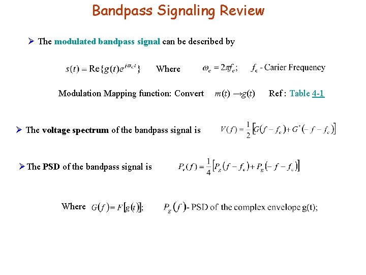
Bandpass Signaling Review Ø The modulated bandpass signal can be described by Where Modulation Mapping function: Convert Ø The voltage spectrum of the bandpass signal is ØThe PSD of the bandpass signal is Where m(t) →g(t) Ref : Table 4 -1
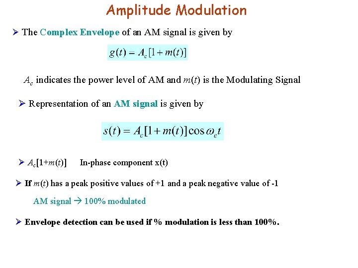
Amplitude Modulation Ø The Complex Envelope of an AM signal is given by Ac indicates the power level of AM and m(t) is the Modulating Signal Ø Representation of an AM signal is given by Ø Ac[1+m(t)] In-phase component x(t) Ø If m(t) has a peak positive values of +1 and a peak negative value of -1 AM signal 100% modulated Ø Envelope detection can be used if % modulation is less than 100%.
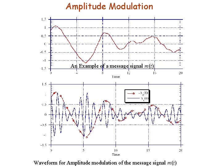
Amplitude Modulation An Example of a message signal m(t) Waveform for Amplitude modulation of the message signal m(t)
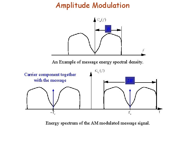
Amplitude Modulation B An Example of message energy spectral density. Carrier component together with the message 2 B Energy spectrum of the AM modulated message signal.

AM – Percentage Modulation Ø Definition: The percentage of positive modulation on an AM signal is Ø The percentage of negative modulation on an AM signal is Ø The percentage of overall modulation is If m(t) has a peak positive values of +1 and a peak negative value of -1 AM signal 100% modulated
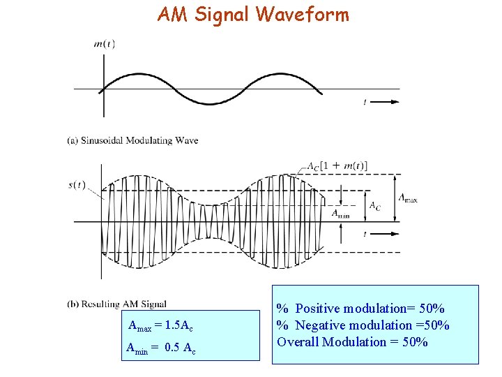
AM Signal Waveform Amax = 1. 5 Ac Amin = 0. 5 Ac % Positive modulation= 50% % Negative modulation =50% Overall Modulation = 50%
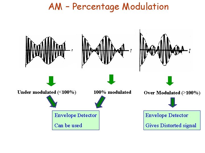
AM – Percentage Modulation Under modulated (<100%) 100% modulated Over Modulated (>100%) Envelope Detector Can be used Gives Distorted signal
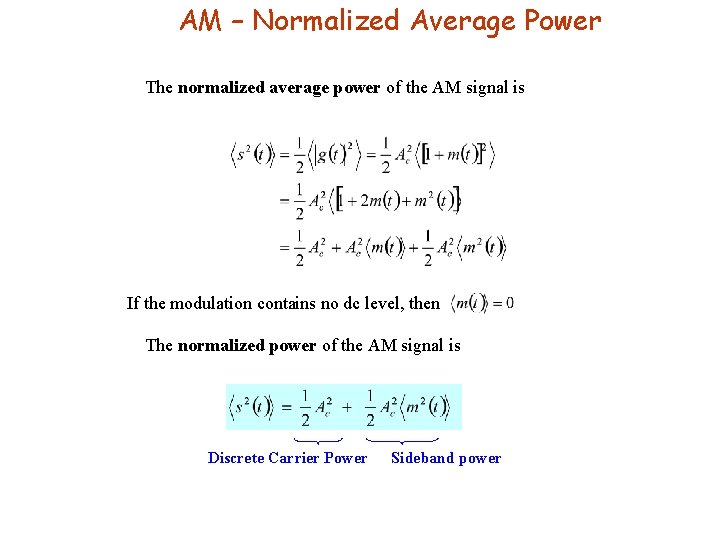
AM – Normalized Average Power The normalized average power of the AM signal is If the modulation contains no dc level, then The normalized power of the AM signal is Discrete Carrier Power Sideband power
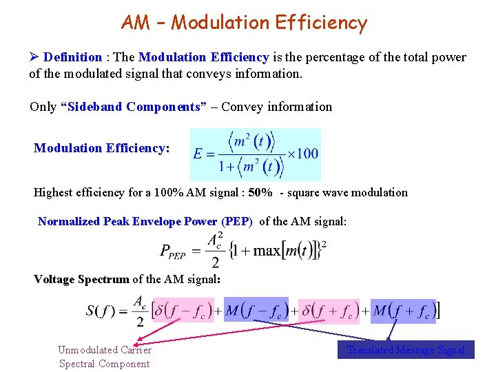
AM – Modulation Efficiency Ø Definition : The Modulation Efficiency is the percentage of the total power of the modulated signal that conveys information. Only “Sideband Components” – Convey information Modulation Efficiency: Highest efficiency for a 100% AM signal : 50% - square wave modulation Normalized Peak Envelope Power (PEP) of the AM signal: Voltage Spectrum of the AM signal: Unmodulated Carrier Spectral Component Translated Message Signal
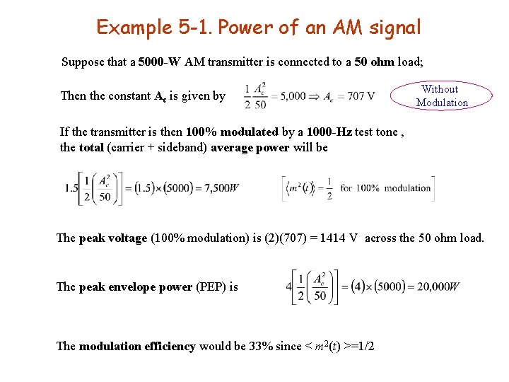
Example 5 -1. Power of an AM signal Suppose that a 5000 -W AM transmitter is connected to a 50 ohm load; Then the constant Ac is given by Without Modulation If the transmitter is then 100% modulated by a 1000 -Hz test tone , the total (carrier + sideband) average power will be The peak voltage (100% modulation) is (2)(707) = 1414 V across the 50 ohm load. The peak envelope power (PEP) is The modulation efficiency would be 33% since < m 2(t) >=1/2
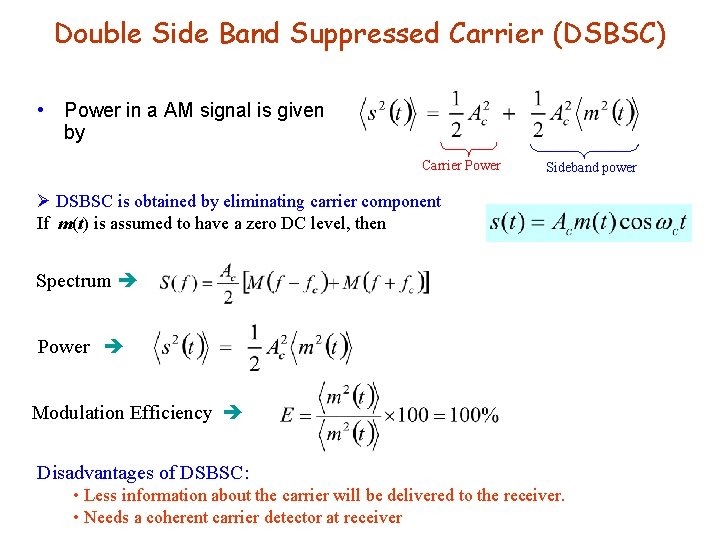
Double Side Band Suppressed Carrier (DSBSC) • Power in a AM signal is given by Carrier Power Sideband power Ø DSBSC is obtained by eliminating carrier component If m(t) is assumed to have a zero DC level, then Spectrum Power Modulation Efficiency Disadvantages of DSBSC: • Less information about the carrier will be delivered to the receiver. • Needs a coherent carrier detector at receiver
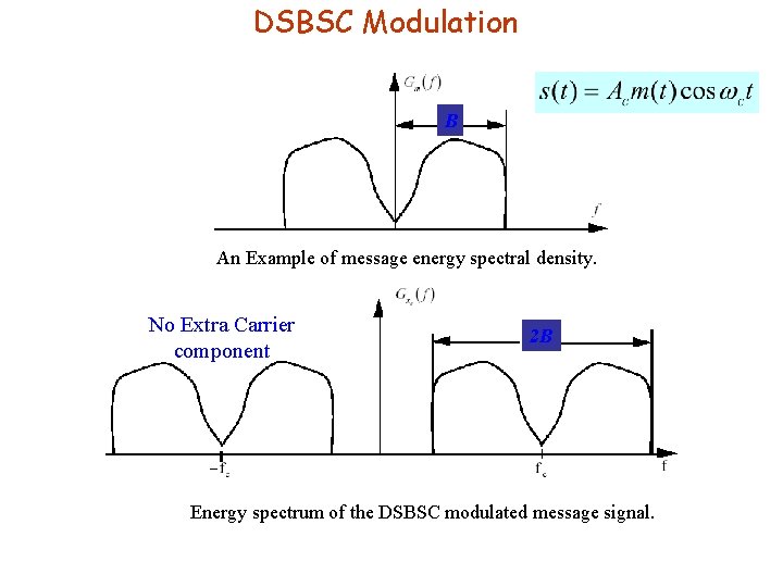
DSBSC Modulation B An Example of message energy spectral density. No Extra Carrier component 2 B Energy spectrum of the DSBSC modulated message signal.
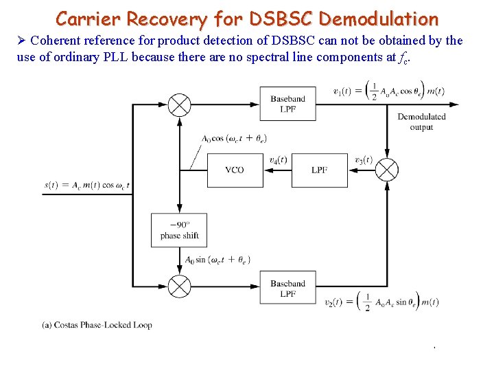
Carrier Recovery for DSBSC Demodulation Ø Coherent reference for product detection of DSBSC can not be obtained by the use of ordinary PLL because there are no spectral line components at fc.
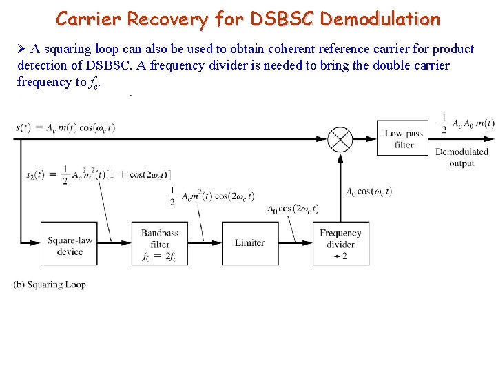
Carrier Recovery for DSBSC Demodulation Ø A squaring loop can also be used to obtain coherent reference carrier for product detection of DSBSC. A frequency divider is needed to bring the double carrier frequency to fc.
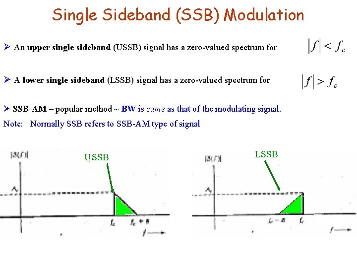
Single Sideband (SSB) Modulation Ø An upper single sideband (USSB) signal has a zero-valued spectrum for Ø A lower single sideband (LSSB) signal has a zero-valued spectrum for Ø SSB-AM – popular method ~ BW is same as that of the modulating signal. Note: Normally SSB refers to SSB-AM type of signal USSB LSSB
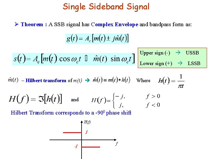
Single Sideband Signal Ø Theorem : A SSB signal has Complex Envelope and bandpass form as: Upper sign (-) Lower sign (+) – Hilbert transform of m(t) Where and Hilbert Transform corresponds to a -900 phase shift H(f) j -j f USSB LSSB
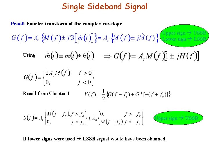
Single Sideband Signal Proof: Fourier transform of the complex envelope Upper sign USSB Lower sign LSSB Using Recall from Chapter 4 Upper sign USSB If lower signs were used LSSB signal would have been obtained
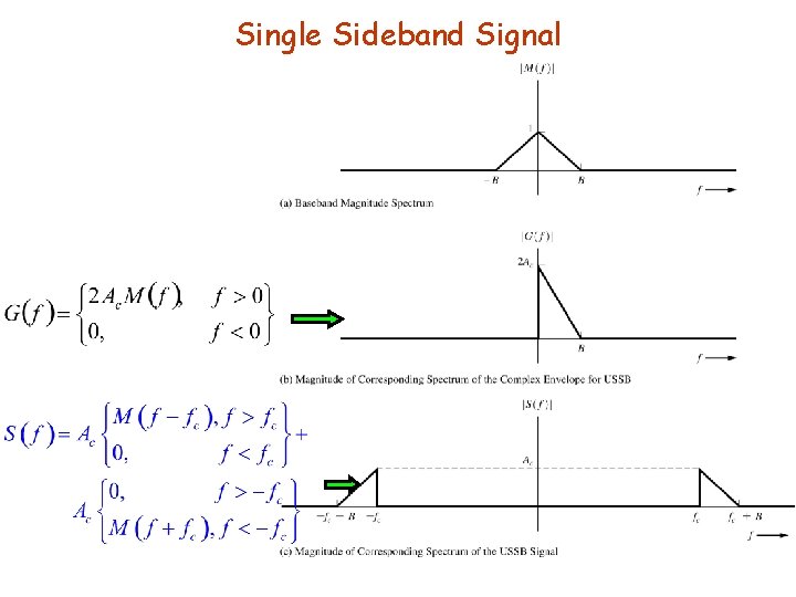
Single Sideband Signal
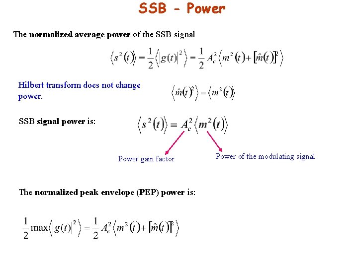
SSB - Power The normalized average power of the SSB signal Hilbert transform does not change power. SSB signal power is: Power gain factor The normalized peak envelope (PEP) power is: Power of the modulating signal

Generation of SSB signals have both AM and PM. The complex envelope of SSB: For the AM component, For the PM component, Advantages of SSB • Superior detected signal-to-noise ratio compared to that of AM • SSB has one-half the bandwidth of AM or DSB-SC signals
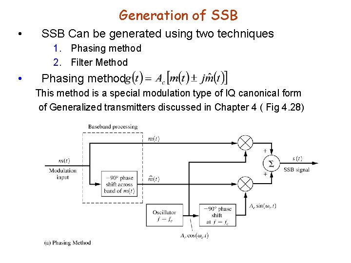
Generation of SSB • SSB Can be generated using two techniques 1. Phasing method 2. Filter Method • Phasing method This method is a special modulation type of IQ canonical form of Generalized transmitters discussed in Chapter 4 ( Fig 4. 28)
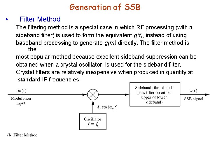
Generation of SSB • Filter Method The filtering method is a special case in which RF processing (with a sideband filter) is used to form the equivalent g(t), instead of using baseband processing to generate g(m) directly. The filter method is the most popular method because excellent sideband suppression can be obtained when a crystal oscillator is used for the sideband filter. Crystal filters are relatively inexpensive when produced in quantity at standard IF frequencies.
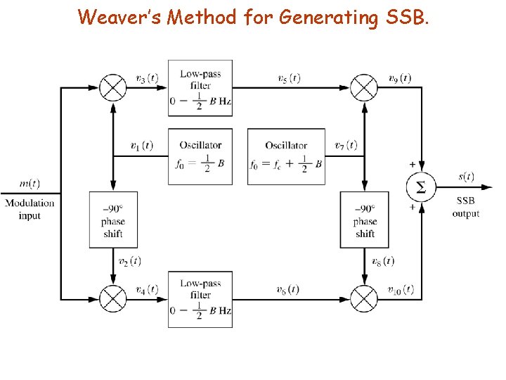
Weaver’s Method for Generating SSB.
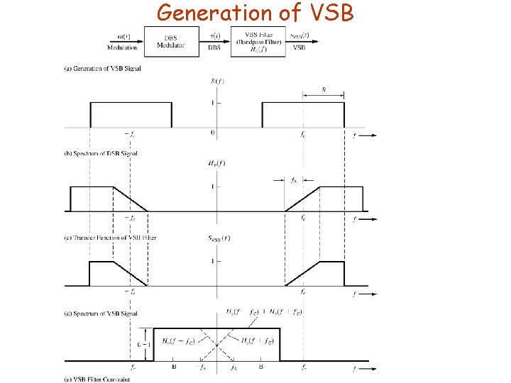
Generation of VSB
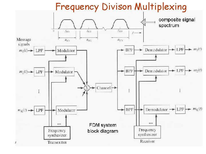
Frequency Divison Multiplexing
AM, FM, and Digital Modulated Systems Ø Ø Ø Phase Modulation (PM) Frequency Modulation (FM) Generation of PM and FM Spectrum of PM and FM Carson’s Rule Narrowband FM

AM and FM Modulation (a) Carrier wave. (b) Sinusoidal modulating signal. (c) Amplitude-modulated signal. (d) Frequency modulated signal.
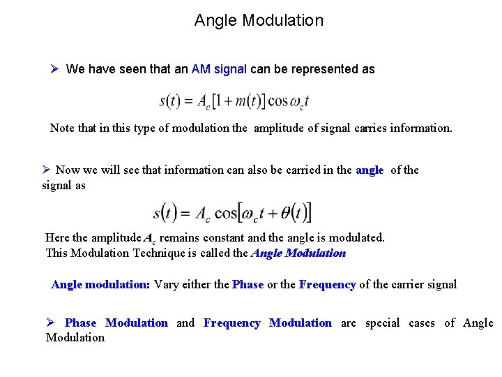
Angle Modulation Ø We have seen that an AM signal can be represented as Note that in this type of modulation the amplitude of signal carries information. Ø Now we will see that information can also be carried in the angle of the signal as Here the amplitude Ac remains constant and the angle is modulated. This Modulation Technique is called the Angle Modulation Angle modulation: Vary either the Phase or the Frequency of the carrier signal Ø Phase Modulation and Frequency Modulation are special cases of Angle Modulation
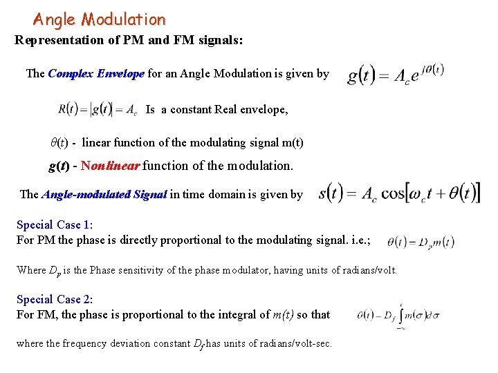
Angle Modulation Representation of PM and FM signals: The Complex Envelope for an Angle Modulation is given by Is a constant Real envelope, θ(t) - linear function of the modulating signal m(t) g(t) - Nonlinear function of the modulation. The Angle-modulated Signal in time domain is given by Special Case 1: For PM the phase is directly proportional to the modulating signal. i. e. ; Where Dp is the Phase sensitivity of the phase modulator, having units of radians/volt. Special Case 2: For FM, the phase is proportional to the integral of m(t) so that where the frequency deviation constant Df has units of radians/volt-sec.
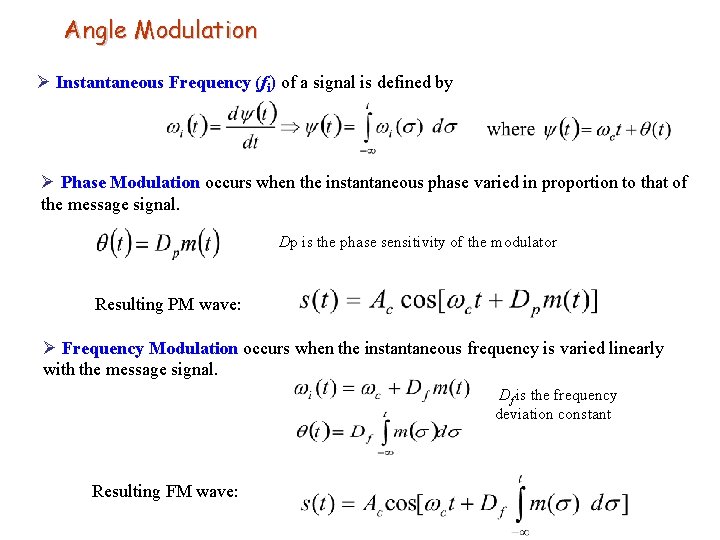
Angle Modulation Ø Instantaneous Frequency (fi) of a signal is defined by Ø Phase Modulation occurs when the instantaneous phase varied in proportion to that of the message signal. Dp is the phase sensitivity of the modulator Resulting PM wave: Ø Frequency Modulation occurs when the instantaneous frequency is varied linearly with the message signal. Df is the frequency deviation constant Resulting FM wave:
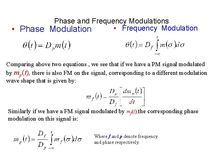
Phase and Frequency Modulations • Frequency Modulation • Phase Modulation Comparing above two equations , we see that if we have a PM signal modulated by mp(t), there is also FM on the signal, corresponding to a different modulation wave shape that is given by: Similarly if we have a FM signal modulated by mf(t), the corresponding phase modulation on this signal is: Where f and p denote frequency and phase respectively.

Generation of FM from PM and vice versa Generation of FM using a Phase Modulator: Integrator Phase Modulator (Carrier Frequency fc) FM Signal Generation of PM using a Frequency Modulator: Differentiator Frequency Modulator (Carrier Frequency fc) PM signal
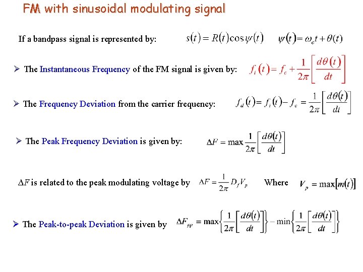
FM with sinusoidal modulating signal If a bandpass signal is represented by: Ø The Instantaneous Frequency of the FM signal is given by: Ø The Frequency Deviation from the carrier frequency: Ø The Peak Frequency Deviation is given by: ∆F is related to the peak modulating voltage by Ø The Peak-to-peak Deviation is given by Where
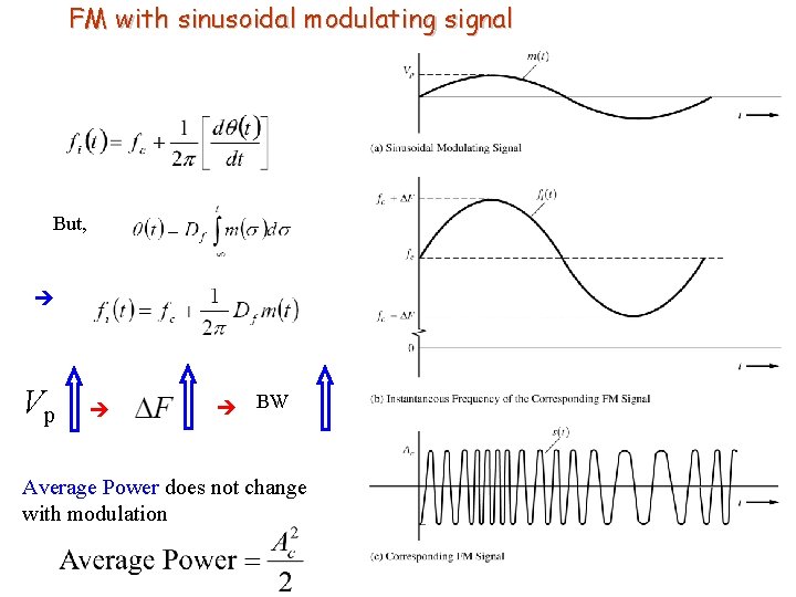
FM with sinusoidal modulating signal But, Vp BW Average Power does not change with modulation
Angle Modulation Advantages: Ø Constant amplitude means Efficient Non-linear Power Amplifiers can be used. Ø Superior signal-to-noise ratio can be achieved (compared to AM) if bandwidth is sufficiently high. Disadvantages: Ø Usually require more bandwidth than AM Ø More complicated hardware
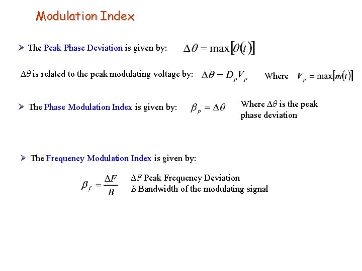
Modulation Index Ø The Peak Phase Deviation is given by: ∆θ is related to the peak modulating voltage by: Ø The Phase Modulation Index is given by: Where ∆θ is the peak phase deviation Ø The Frequency Modulation Index is given by: ∆F Peak Frequency Deviation B Bandwidth of the modulating signal
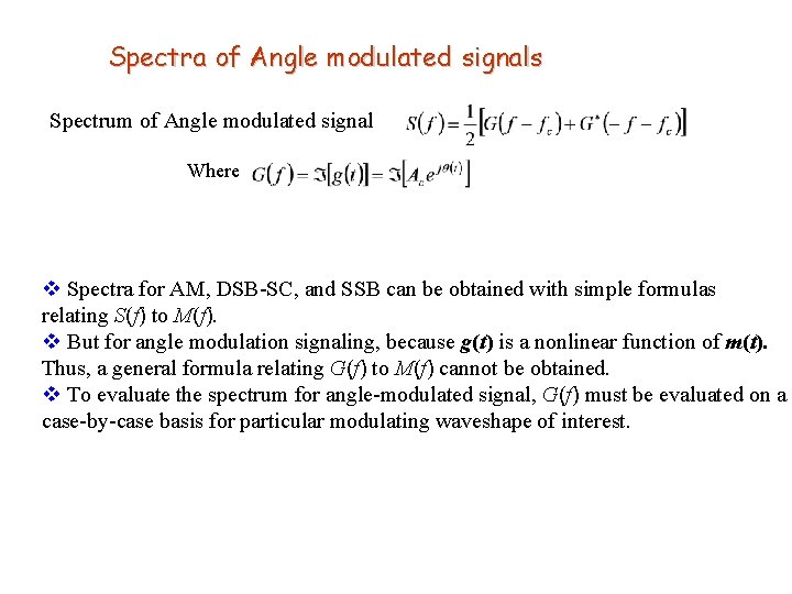
Spectra of Angle modulated signals Spectrum of Angle modulated signal Where v Spectra for AM, DSB-SC, and SSB can be obtained with simple formulas relating S(f) to M(f). v But for angle modulation signaling, because g(t) is a nonlinear function of m(t). Thus, a general formula relating G(f) to M(f) cannot be obtained. v To evaluate the spectrum for angle-modulated signal, G(f) must be evaluated on a case-by-case basis for particular modulating waveshape of interest.

Spectrum of PM or FM Signal with Sinusoidal Modulating Signal Ø Assume that the modulation on the PM signal is Then Where is the phase Modulation Index. Same θ(t) could also be obtained if FM were used where and The peak frequency deviation would be The Complex Envelope is: which is periodic with period
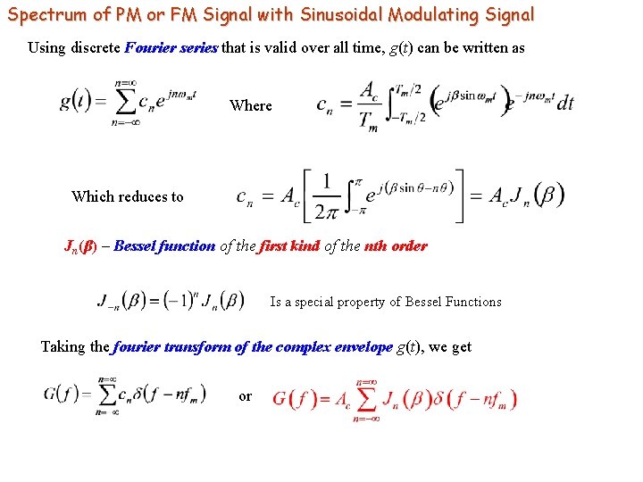
Spectrum of PM or FM Signal with Sinusoidal Modulating Signal Using discrete Fourier series that is valid over all time, g(t) can be written as Where Which reduces to Jn(β) – Bessel function of the first kind of the nth order Is a special property of Bessel Functions Taking the fourier transform of the complex envelope g(t), we get or
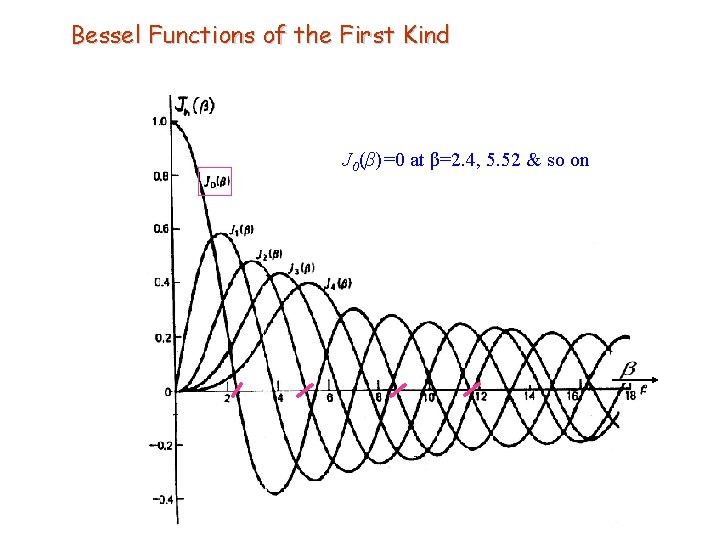
Bessel Functions of the First Kind J 0(β)=0 at β=2. 4, 5. 52 & so on
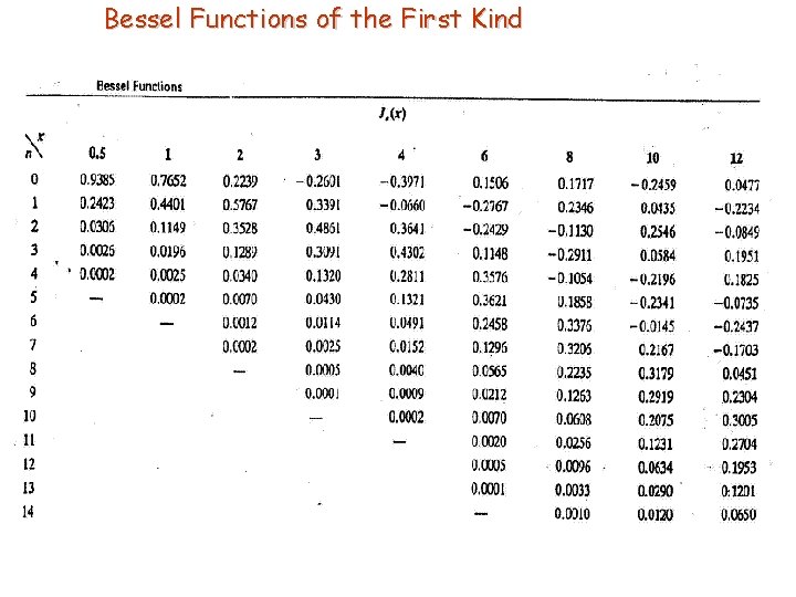
Bessel Functions of the First Kind
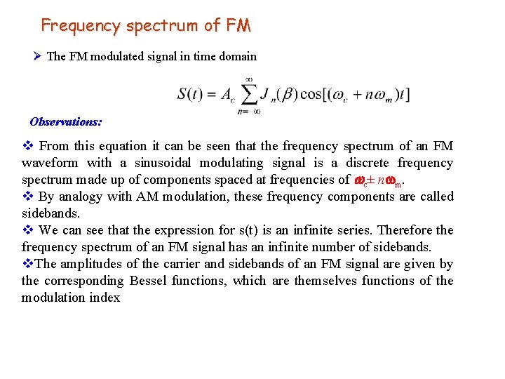
Frequency spectrum of FM Ø The FM modulated signal in time domain Observations: v From this equation it can be seen that the frequency spectrum of an FM waveform with a sinusoidal modulating signal is a discrete frequency spectrum made up of components spaced at frequencies of c± n m. v By analogy with AM modulation, these frequency components are called sidebands. v We can see that the expression for s(t) is an infinite series. Therefore the frequency spectrum of an FM signal has an infinite number of sidebands. v. The amplitudes of the carrier and sidebands of an FM signal are given by the corresponding Bessel functions, which are themselves functions of the modulation index
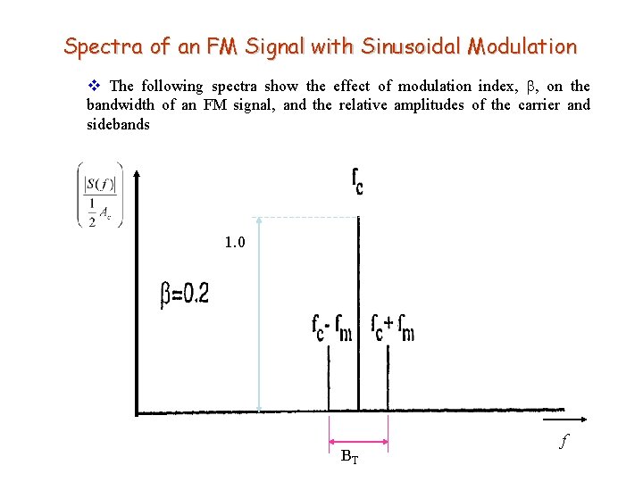
Spectra of an FM Signal with Sinusoidal Modulation v The following spectra show the effect of modulation index, , on the bandwidth of an FM signal, and the relative amplitudes of the carrier and sidebands 1. 0 BT f
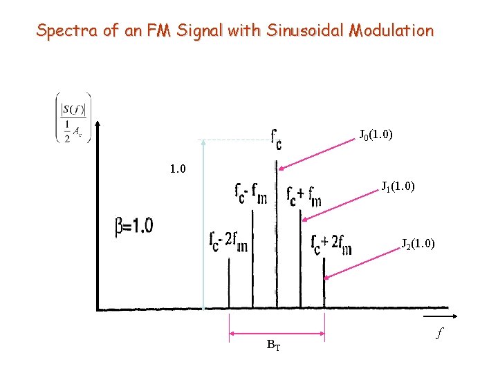
Spectra of an FM Signal with Sinusoidal Modulation J 0(1. 0) 1. 0 J 1(1. 0) J 2(1. 0) BT f
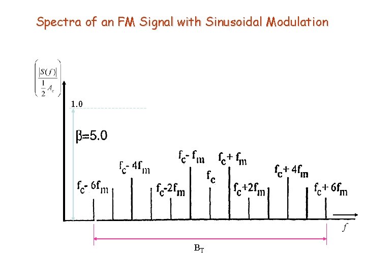
Spectra of an FM Signal with Sinusoidal Modulation 1. 0 f BT
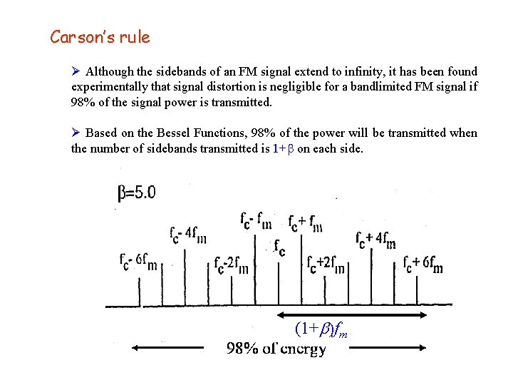
Carson’s rule Ø Although the sidebands of an FM signal extend to infinity, it has been found experimentally that signal distortion is negligible for a bandlimited FM signal if 98% of the signal power is transmitted. Ø Based on the Bessel Functions, 98% of the power will be transmitted when the number of sidebands transmitted is 1+ on each side. (1+b)fm
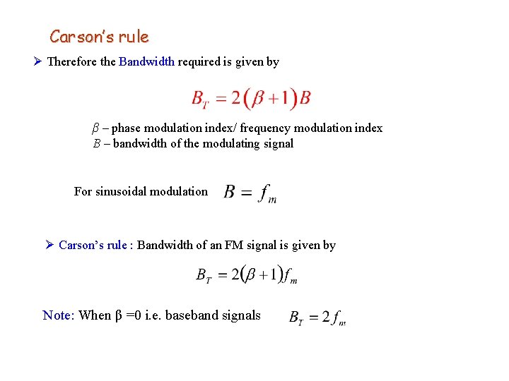
Carson’s rule Ø Therefore the Bandwidth required is given by β – phase modulation index/ frequency modulation index B – bandwidth of the modulating signal For sinusoidal modulation Ø Carson’s rule : Bandwidth of an FM signal is given by Note: When β =0 i. e. baseband signals
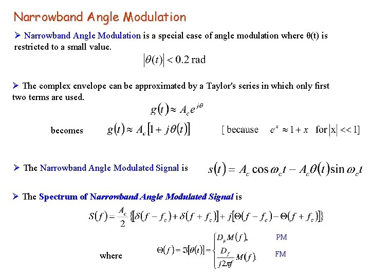
Narrowband Angle Modulation Ø Narrowband Angle Modulation is a special case of angle modulation where θ(t) is restricted to a small value. Ø The complex envelope can be approximated by a Taylor's series in which only first two terms are used. becomes Ø The Narrowband Angle Modulated Signal is Ø The Spectrum of Narrowband Angle Modulated Signal is PM where FM
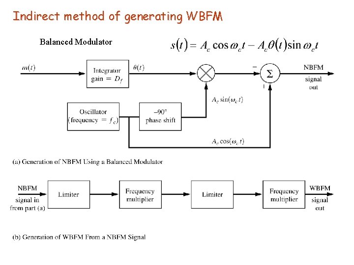
Indirect method of generating WBFM Balanced Modulator
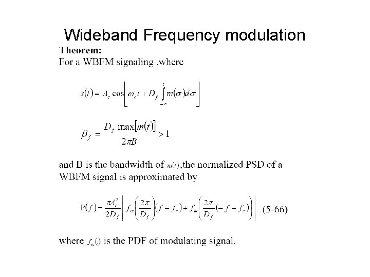
Wideband Frequency modulation
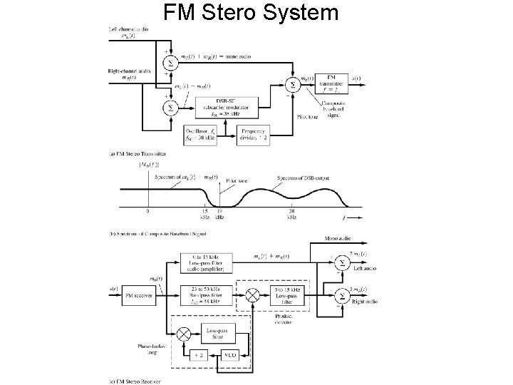
FM Stero System
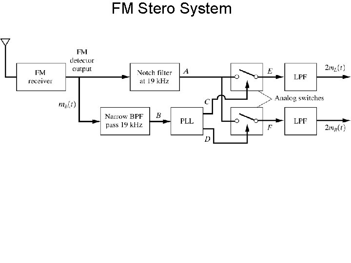
FM Stero System
AM, FM, and Digital Modulated Systems Ø Ø Binary Bandpass Signalling Techniques OOK BPSK FSK
![Binary Bandpass Signaling techniques Ø On–Off keying (OOK) [amplitude shift keying (ASK)] - Consists](http://slidetodoc.com/presentation_image_h2/f266b1eb432c3f1e17a32030c19bfd48/image-56.jpg "Binary Bandpass Signaling techniques Ø On–Off keying (OOK) [amplitude shift keying (ASK)] - Consists")
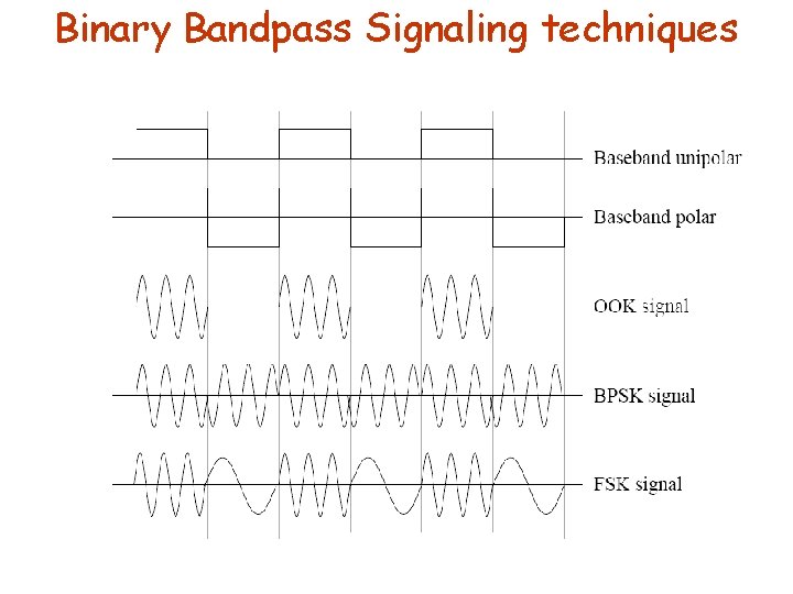
Binary Bandpass Signaling techniques Ø On–Off keying (OOK) [amplitude shift keying (ASK)] - Consists of keying (switching) a carrier sinusoid on and off with a unipolar binary signal. - Morse code radio transmission is an example of this technique. - OOK was one of the first modulation techniques to be used and precedes communication systems. analog Ø Binary Phase-Shift Keying (BPSK) - Consists of shifting the phase of a sinusoidal carrier 0 o or 180 o with a unipolar binary signal. - BPSK is equivalent to PM signaling with a digital waveform. Ø Frequency-Shift Keying (FSK) - Consists of shifting the frequency of a sinusoidal carrier from a mark frequency (binary 1) to a space frequency (binary 0), according to the baseband digital signal. - FSK is identical to modulating an FM carrier with a binary digital signal.
Binary Bandpass Signaling techniques
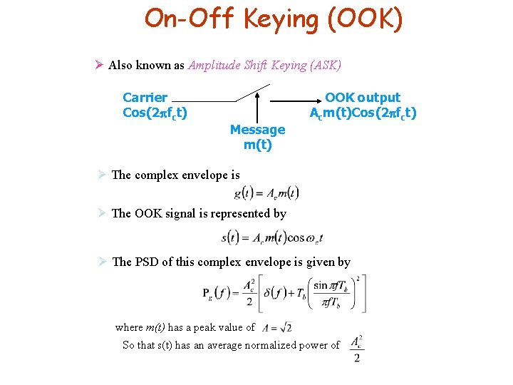
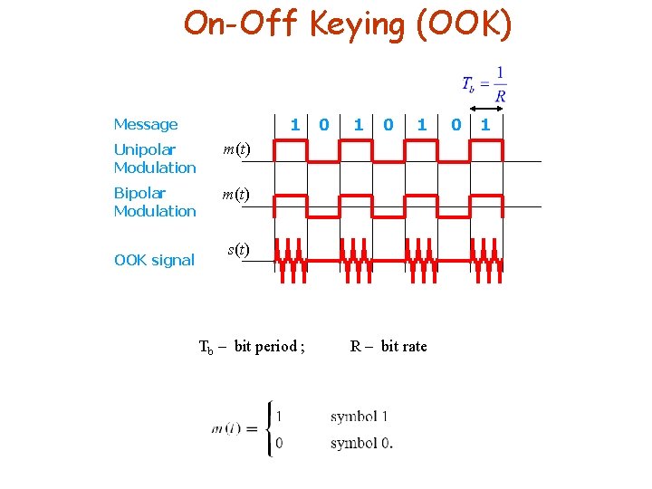
On-Off Keying (OOK) Ø Also known as Amplitude Shift Keying (ASK) Carrier Cos(2 fct) Message m(t) OOK output Acm(t)Cos(2 fct) Ø The complex envelope is Ø The OOK signal is represented by Ø The PSD of this complex envelope is given by where m(t) has a peak value of So that s(t) has an average normalized power of
On-Off Keying (OOK) 1 Message Unipolar Modulation m(t) Bipolar Modulation m(t) OOK signal 0 1 s(t) Tb – bit period ; R – bit rate 0 1
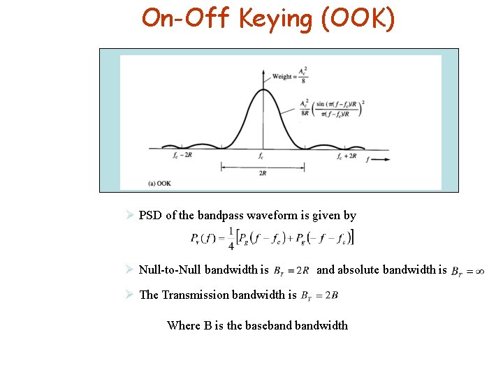
On-Off Keying (OOK) Ø PSD of the bandpass waveform is given by Ø Null-to-Null bandwidth is and absolute bandwidth is Ø The Transmission bandwidth is Where B is the basebandwidth
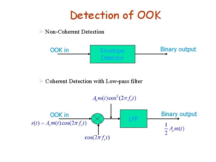
Detection of OOK Ø Non-Coherent Detection OOK in Binary output Envelope Detector Ø Coherent Detection with Low-pass filter OOK in LPF Binary output
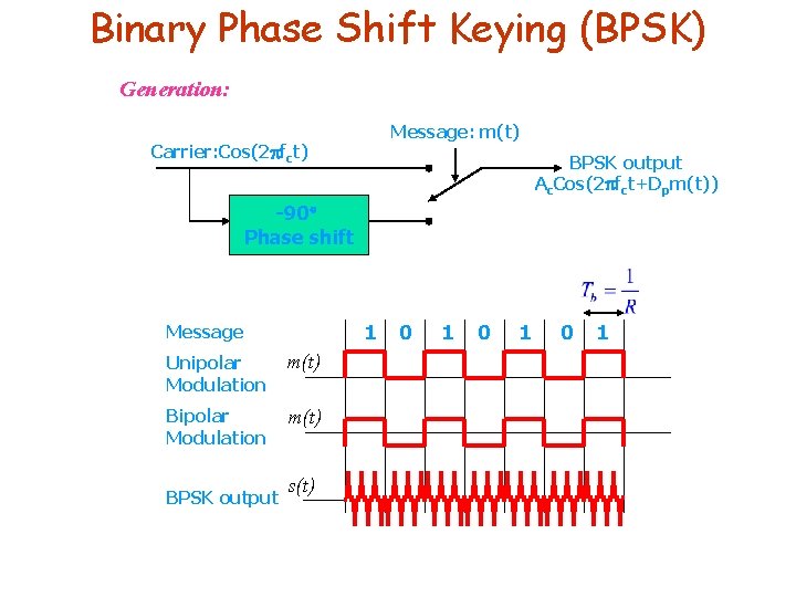
Binary Phase Shift Keying (BPSK) Generation: Message: m(t) Carrier: Cos(2 fct) BPSK output Ac. Cos(2 fct+Dpm(t)) -90 Phase shift 1 Message Unipolar Modulation m(t) BPSK output s(t) 0 1 0 1

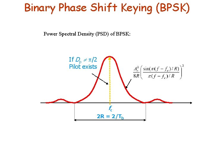
Binary Phase Shift Keying (BPSK) Ø The BPSK signal is represented by let pilot carrier term data term Ø The level of the pilot carrier term is set by the value of the peak deviation Ø The digital modulation index ‘h’ is given by 2∆θ – maximum peak-to-peak deviation during time Ts Ø If Dp is small, then there is little power in data term & more in pilot term Ø To maximize performance (minimum probability of error) Optimum case : BPSK signal :
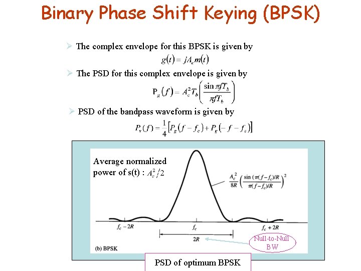
Binary Phase Shift Keying (BPSK) Ø The complex envelope for this BPSK is given by Ø The PSD for this complex envelope is given by Ø PSD of the bandpass waveform is given by Average normalized power of s(t) : Null-to-Null BW PSD of optimum BPSK
Binary Phase Shift Keying (BPSK) Power Spectral Density (PSD) of BPSK: If Dp /2 Pilot exists fc 2 R = 2/Tb
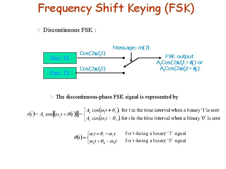
Frequency Shift Keying (FSK) Ø Discontinuous FSK : Osc. f 1 Osc. f 2 Cos(2 f 1 t) Cos(2 f 2 t) Message: m(t) FSK output Ac. Cos(2 f 1 t+ 1) or Ac. Cos(2 f 2 t+ 2) Ø The discontinuous-phase FSK signal is represented by for t during a binary ‘ 1’ signal for t during a binary ‘ 0’ signal
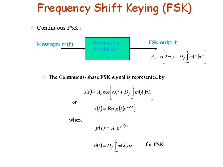
Frequency Shift Keying (FSK) Ø Continuous FSK : Message: m(t) Frequency Modulator fc FSK output Ø The Continuous-phase FSK signal is represented by or where for FSK

Frequency Shift Keying (FSK) 1 Message Unipolar Modulation m(t) Bipolar Modulation m(t) 0 1 0 1 s(t) FSK output (Discontinuous) FSK output (Continuous) s(t) Mark(binary 1) frequency: f 1 Space(binary 0) frequency: f 2
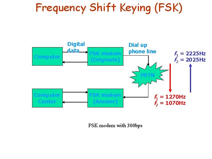
Frequency Shift Keying (FSK) Computer Digital data FSK modem (Originate) Dial up phone line f 1 = 2225 Hz f 2 = 2025 Hz PSTN Computer Center FSK modem (Answer) FSK modem with 300 bps f 1 = 1270 Hz f 2 = 1070 Hz

END
- Slides: 70