154 Topic 5 1 Modeling Stated Preference Data

1/54: Topic 5. 1 – Modeling Stated Preference Data Microeconometric Modeling William Greene Stern School of Business New York University New York NY USA 5. 1 Modeling Stated Preference Data

2/54: Topic 5. 1 – Modeling Stated Preference Data Concepts • • Revealed Preference Stated Preference Attribute Nonattendance Random Utility Attribute Space Experimental Design Choice Experiment Environmental Attitude Models • • • Multinomial Logit Model Latent Class MNL Nested Logit Mixed Logit Error Components Logit

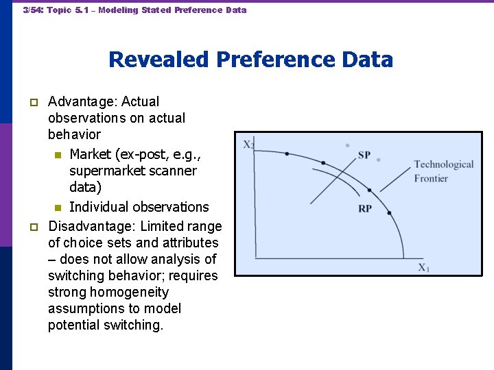
3/54: Topic 5. 1 – Modeling Stated Preference Data Revealed Preference Data p p Advantage: Actual observations on actual behavior n Market (ex-post, e. g. , supermarket scanner data) n Individual observations Disadvantage: Limited range of choice sets and attributes – does not allow analysis of switching behavior; requires strong homogeneity assumptions to model potential switching.

4/54: Topic 5. 1 – Modeling Stated Preference Data p p Disadvantages n Purely hypothetical – does the subject take it seriously? n No necessary anchor to real market situations n Vast heterogeneity across individuals n E. g. , contingent valuation Advantage n Analysis of person specific behavior, e. g. , switching n Modeling cross section heterogeneity

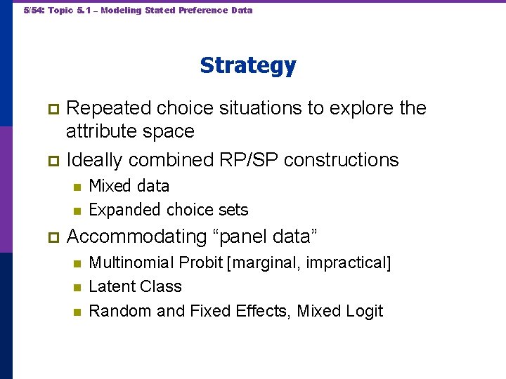
5/54: Topic 5. 1 – Modeling Stated Preference Data Strategy Repeated choice situations to explore the attribute space p Ideally combined RP/SP constructions p n n p Mixed data Expanded choice sets Accommodating “panel data” n n n Multinomial Probit [marginal, impractical] Latent Class Random and Fixed Effects, Mixed Logit

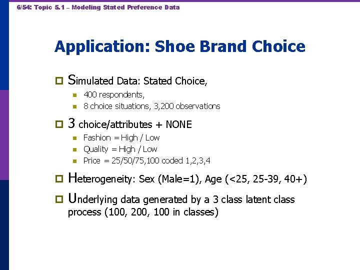
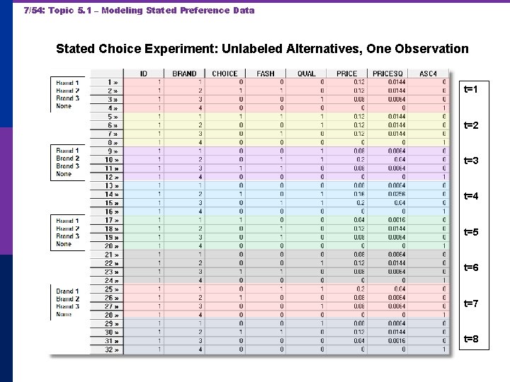
6/54: Topic 5. 1 – Modeling Stated Preference Data Application: Shoe Brand Choice p Simulated Data: Stated Choice, n n p 400 respondents, 8 choice situations, 3, 200 observations 3 choice/attributes + NONE n n n Fashion = High / Low Quality = High / Low Price = 25/50/75, 100 coded 1, 2, 3, 4 Heterogeneity: Sex (Male=1), Age (<25, 25 -39, 40+) p Underlying data generated by a 3 class latent class p process (100, 200, 100 in classes)

7/54: Topic 5. 1 – Modeling Stated Preference Data Stated Choice Experiment: Unlabeled Alternatives, One Observation t=1 t=2 t=3 t=4 t=5 t=6 t=7 t=8

8/54: Topic 5. 1 – Modeling Stated Preference Data Application: Pregnancy Care Guidelines

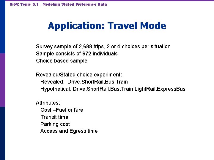
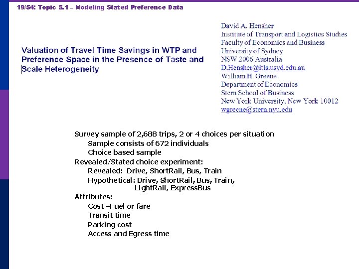
9/54: Topic 5. 1 – Modeling Stated Preference Data Application: Travel Mode Survey sample of 2, 688 trips, 2 or 4 choices per situation Sample consists of 672 individuals Choice based sample Revealed/Stated choice experiment: Revealed: Drive, Short. Rail, Bus, Train Hypothetical: Drive, Short. Rail, Bus, Train, Light. Rail, Express. Bus Attributes: Cost –Fuel or fare Transit time Parking cost Access and Egress time

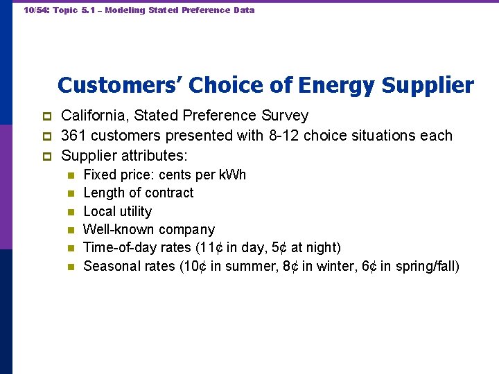
10/54: Topic 5. 1 – Modeling Stated Preference Data Customers’ Choice of Energy Supplier p p p California, Stated Preference Survey 361 customers presented with 8 -12 choice situations each Supplier attributes: n n n Fixed price: cents per k. Wh Length of contract Local utility Well-known company Time-of-day rates (11¢ in day, 5¢ at night) Seasonal rates (10¢ in summer, 8¢ in winter, 6¢ in spring/fall)

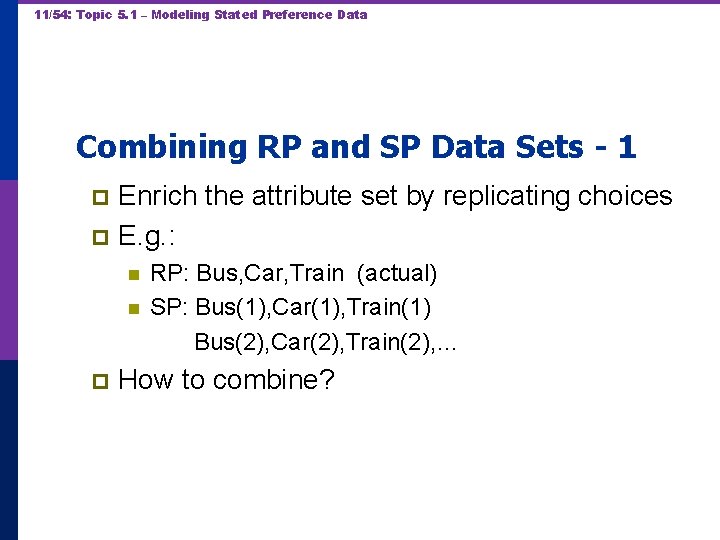
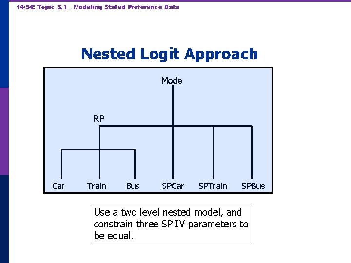
11/54: Topic 5. 1 – Modeling Stated Preference Data Combining RP and SP Data Sets - 1 Enrich the attribute set by replicating choices p E. g. : p n n p RP: Bus, Car, Train (actual) SP: Bus(1), Car(1), Train(1) Bus(2), Car(2), Train(2), … How to combine?

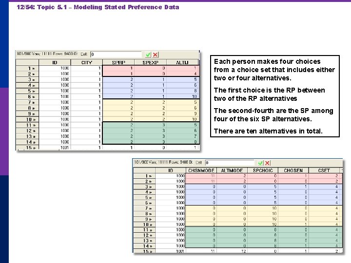
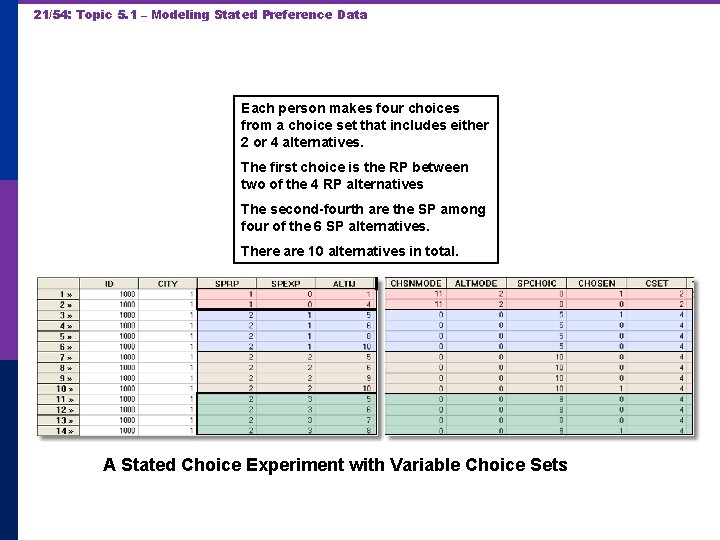
12/54: Topic 5. 1 – Modeling Stated Preference Data Each person makes four choices from a choice set that includes either two or four alternatives. The first choice is the RP between two of the RP alternatives The second-fourth are the SP among four of the six SP alternatives. There are ten alternatives in total.

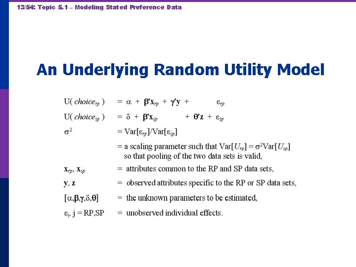
13/54: Topic 5. 1 – Modeling Stated Preference Data An Underlying Random Utility Model

14/54: Topic 5. 1 – Modeling Stated Preference Data Nested Logit Approach Mode RP Car Train Bus SPCar SPTrain SPBus Use a two level nested model, and constrain three SP IV parameters to be equal.

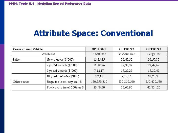
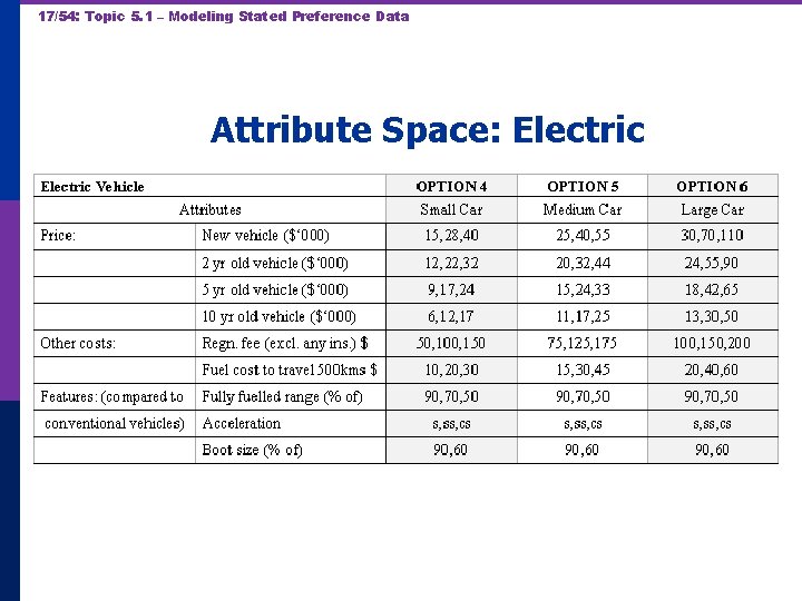
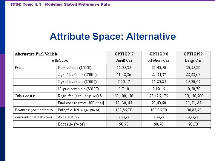
15/54: Topic 5. 1 – Modeling Stated Preference Data Enriched Data Set – Vehicle Choice Choosing between Conventional, Electric and LPG/CNG Vehicles in Single-Vehicle Households David A. Hensher Institute of Transport Studies School of Business The University of Sydney NSW 2006 Australia p p p William H. Greene Department of Economics Stern School of Business New York University New York USA Conventional, Electric, Alternative 1, 400 Sydney Households Automobile choice survey RP + 3 SP fuel classes Nested logit – 2 level approach – to handle the scaling issue

16/54: Topic 5. 1 – Modeling Stated Preference Data Attribute Space: Conventional

17/54: Topic 5. 1 – Modeling Stated Preference Data Attribute Space: Electric

18/54: Topic 5. 1 – Modeling Stated Preference Data Attribute Space: Alternative

19/54: Topic 5. 1 – Modeling Stated Preference Data Survey sample of 2, 688 trips, 2 or 4 choices per situation Sample consists of 672 individuals Choice based sample Revealed/Stated choice experiment: Revealed: Drive, Short. Rail, Bus, Train Hypothetical: Drive, Short. Rail, Bus, Train, Light. Rail, Express. Bus Attributes: Cost –Fuel or fare Transit time Parking cost Access and Egress time

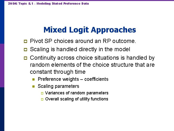
20/54: Topic 5. 1 – Modeling Stated Preference Data Mixed Logit Approaches p p p Pivot SP choices around an RP outcome. Scaling is handled directly in the model Continuity across choice situations is handled by random elements of the choice structure that are constant through time n n Preference weights – coefficients Scaling parameters p p Variances of random parameters Overall scaling of utility functions

21/54: Topic 5. 1 – Modeling Stated Preference Data Each person makes four choices from a choice set that includes either 2 or 4 alternatives. The first choice is the RP between two of the 4 RP alternatives The second-fourth are the SP among four of the 6 SP alternatives. There are 10 alternatives in total. A Stated Choice Experiment with Variable Choice Sets

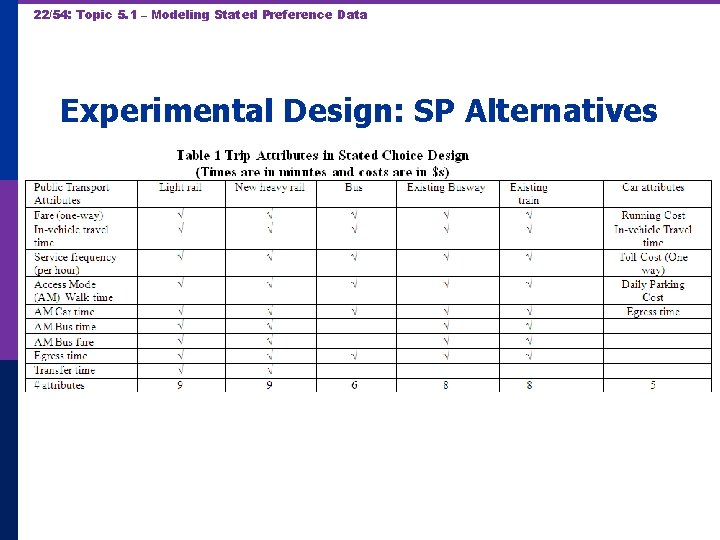
22/54: Topic 5. 1 – Modeling Stated Preference Data Experimental Design: SP Alternatives

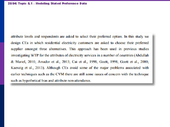
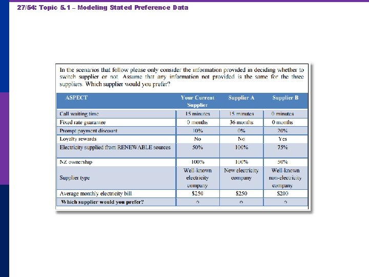
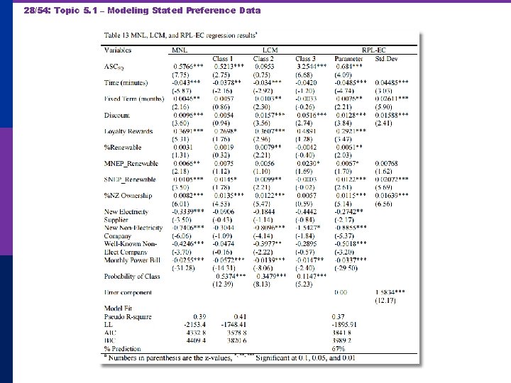
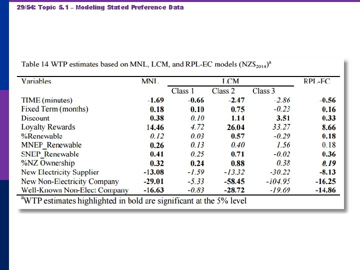
23/54: Topic 5. 1 – Modeling Stated Preference Data Willingness to Pay for Green Energy

24/54: Topic 5. 1 – Modeling Stated Preference Data

25/54: Topic 5. 1 – Modeling Stated Preference Data

26/54: Topic 5. 1 – Modeling Stated Preference Data

27/54: Topic 5. 1 – Modeling Stated Preference Data

28/54: Topic 5. 1 – Modeling Stated Preference Data

29/54: Topic 5. 1 – Modeling Stated Preference Data

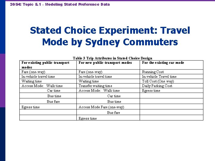
30/54: Topic 5. 1 – Modeling Stated Preference Data Stated Choice Experiment: Travel Mode by Sydney Commuters

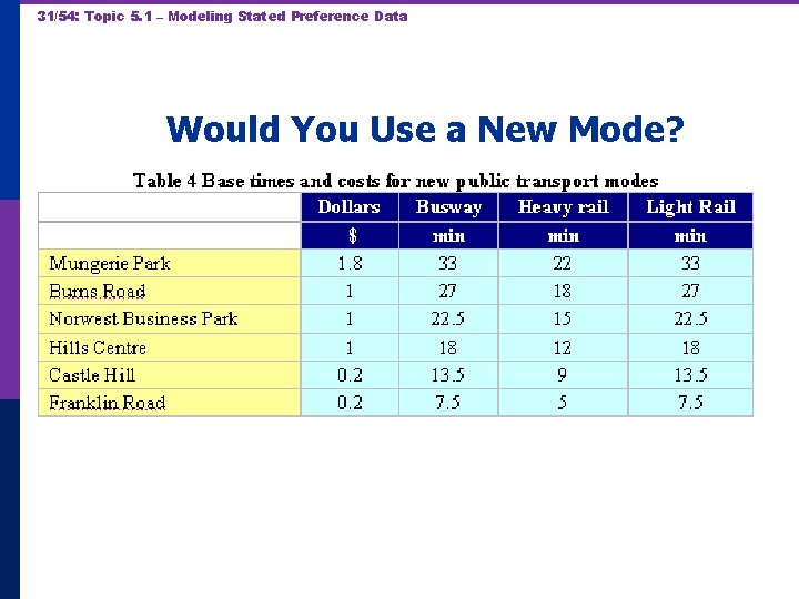
31/54: Topic 5. 1 – Modeling Stated Preference Data Would You Use a New Mode?

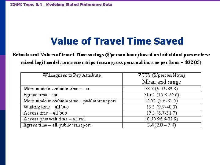
32/54: Topic 5. 1 – Modeling Stated Preference Data Value of Travel Time Saved

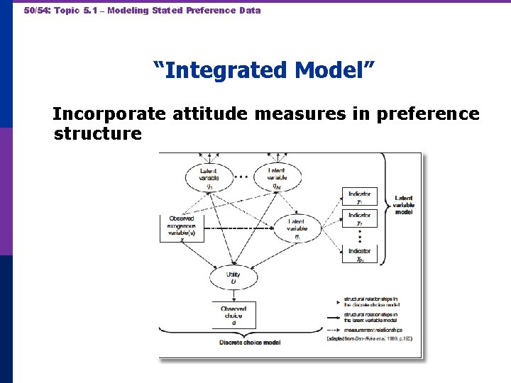
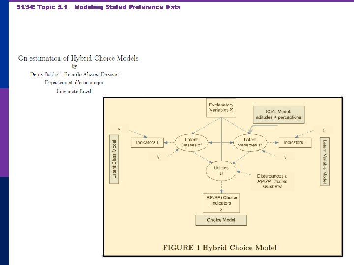
33/54: Topic 5. 1 – Modeling Stated Preference Data Hybrid Choice Models p Incorporates latent variables in choice model p Extends development of discrete choice model to incorporate other aspects of preference structure of the chooser p Develops endogeneity of the preference structure.

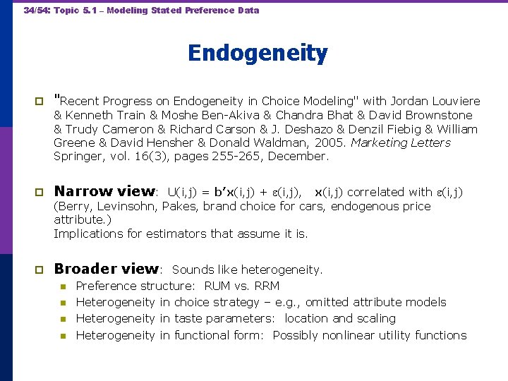
34/54: Topic 5. 1 – Modeling Stated Preference Data Endogeneity p "Recent Progress on Endogeneity in Choice Modeling" with Jordan Louviere & Kenneth Train & Moshe Ben-Akiva & Chandra Bhat & David Brownstone & Trudy Cameron & Richard Carson & J. Deshazo & Denzil Fiebig & William Greene & David Hensher & Donald Waldman, 2005. Marketing Letters Springer, vol. 16(3), pages 255 -265, December. p Narrow view: p Broader view: U(i, j) = b’x(i, j) + (i, j), x(i, j) correlated with (i, j) (Berry, Levinsohn, Pakes, brand choice for cars, endogenous price attribute. ) Implications for estimators that assume it is. n n Sounds like heterogeneity. Preference structure: RUM vs. RRM Heterogeneity in choice strategy – e. g. , omitted attribute models Heterogeneity in taste parameters: location and scaling Heterogeneity in functional form: Possibly nonlinear utility functions

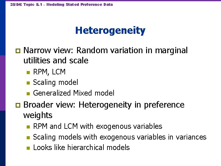
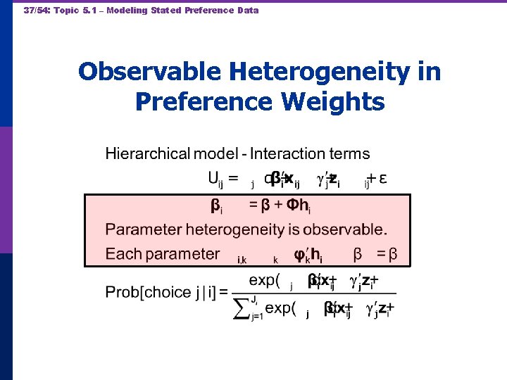
35/54: Topic 5. 1 – Modeling Stated Preference Data Heterogeneity p Narrow view: Random variation in marginal utilities and scale n n n p RPM, LCM Scaling model Generalized Mixed model Broader view: Heterogeneity in preference weights n n n RPM and LCM with exogenous variables Scaling models with exogenous variables in variances Looks like hierarchical models

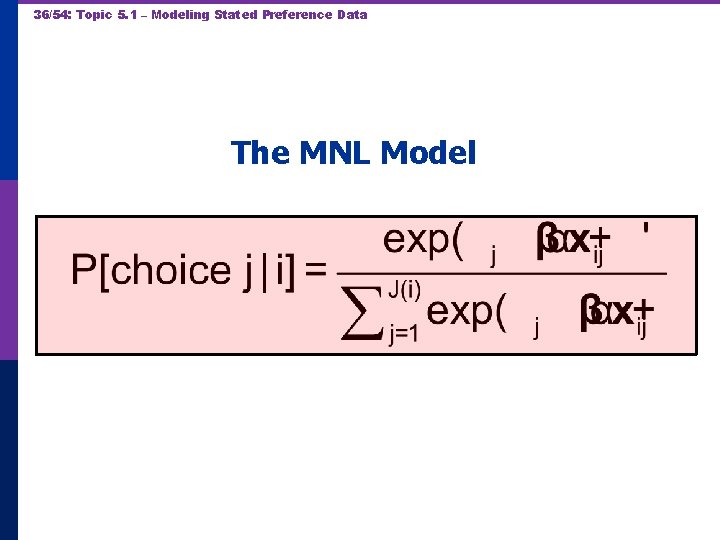
36/54: Topic 5. 1 – Modeling Stated Preference Data The MNL Model

37/54: Topic 5. 1 – Modeling Stated Preference Data Observable Heterogeneity in Preference Weights

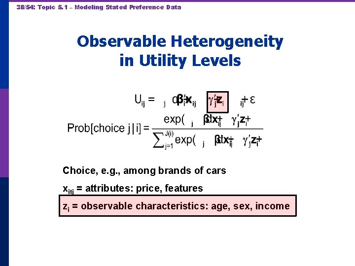
38/54: Topic 5. 1 – Modeling Stated Preference Data Observable Heterogeneity in Utility Levels Choice, e. g. , among brands of cars xitj = attributes: price, features zi = observable characteristics: age, sex, income

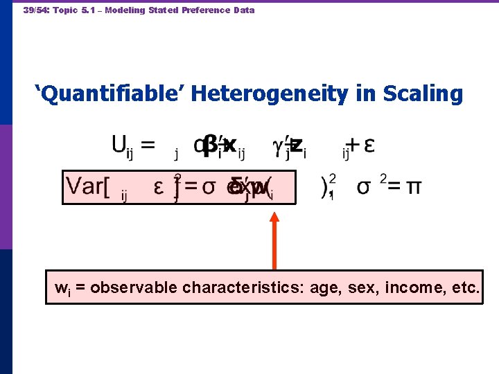
39/54: Topic 5. 1 – Modeling Stated Preference Data ‘Quantifiable’ Heterogeneity in Scaling wi = observable characteristics: age, sex, income, etc.

40/54: Topic 5. 1 – Modeling Stated Preference Data Unobserved Heterogeneity in Scaling

41/54: Topic 5. 1 – Modeling Stated Preference Data A Helpful Way to View Hybrid Choice Models p Adding attitude variables to the choice model p In some formulations, it makes them look like random parameter models

42/54: Topic 5. 1 – Modeling Stated Preference Data Unbservable Heterogeneity in Utility Levels and Other Preference Indicators

43/54: Topic 5. 1 – Modeling Stated Preference Data

44/54: Topic 5. 1 – Modeling Stated Preference Data

45/54: Topic 5. 1 – Modeling Stated Preference Data

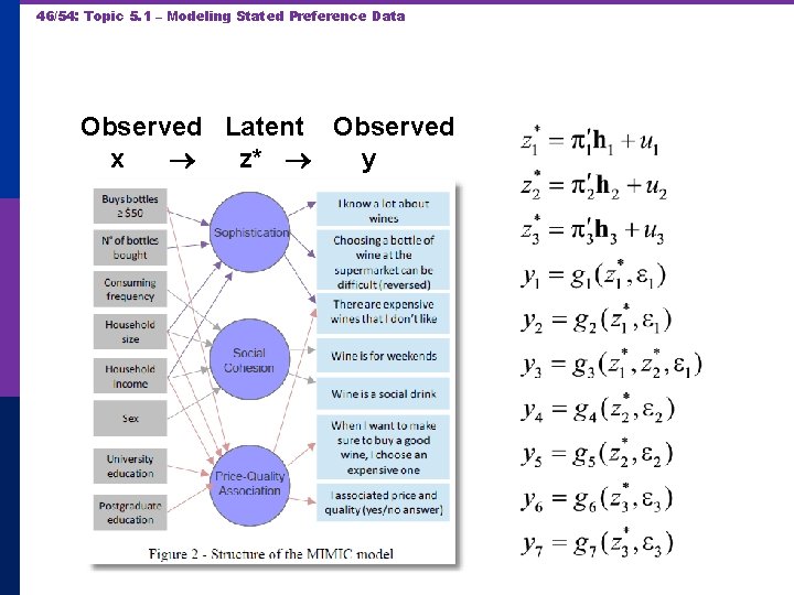
46/54: Topic 5. 1 – Modeling Stated Preference Data Observed Latent Observed x z* y

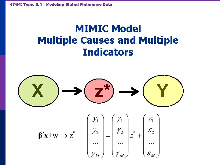
47/54: Topic 5. 1 – Modeling Stated Preference Data MIMIC Model Multiple Causes and Multiple Indicators X z* Y

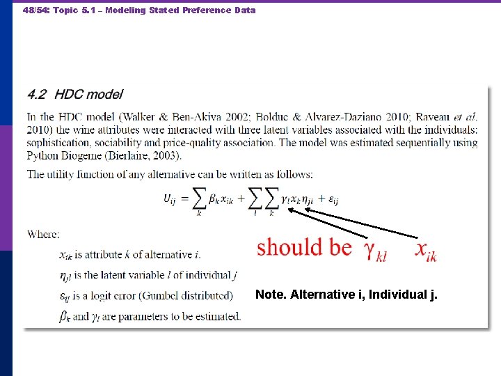
48/54: Topic 5. 1 – Modeling Stated Preference Data Note. Alternative i, Individual j.

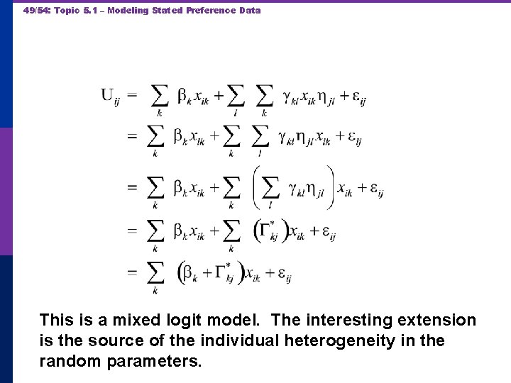
49/54: Topic 5. 1 – Modeling Stated Preference Data This is a mixed logit model. The interesting extension is the source of the individual heterogeneity in the random parameters.

50/54: Topic 5. 1 – Modeling Stated Preference Data “Integrated Model” Incorporate attitude measures in preference structure

51/54: Topic 5. 1 – Modeling Stated Preference Data

52/54: Topic 5. 1 – Modeling Stated Preference Data p p p Swait, J. , “A Structural Equation Model of Latent Segmentation and Product Choice for Cross Sectional Revealed Preference Choice Data, ” Journal of Retailing and Consumer Services, 1994 Bahamonde-Birke and Ortuzar, J. , “On the Variabiity of Hybrid Discrete Choice Models, Transportmetrica, 2012 Vij, A. and J. Walker, “Preference Endogeneity in Discrete Choice Models, ” TRB, 2013 Sener, I. , M. Pendalaya, R. , C. Bhat, “Accommodating Spatial Correlation Across Choice Alternatives in Discrete Choice Models: An Application to Modeling Residential Location Choice Behavior, ” Journal of Transport Geography, 2011 Palma, D. , Ortuzar, J. , G. Casaubon, L. Rizzi, Agosin, E. , “Measuring Consumer Preferences Using Hybrid Discrete Choice Models, ” 2013 Daly, A. , Hess, S. , Patruni, B. , Potoglu, D. , Rohr, C. , “Using Ordered Attitudinal Indicators in a Latent Variable Choice Model: A Study of the Impact of Security on Rail Travel Behavior”