1 PCP Proof Map In previous lectures 3

1

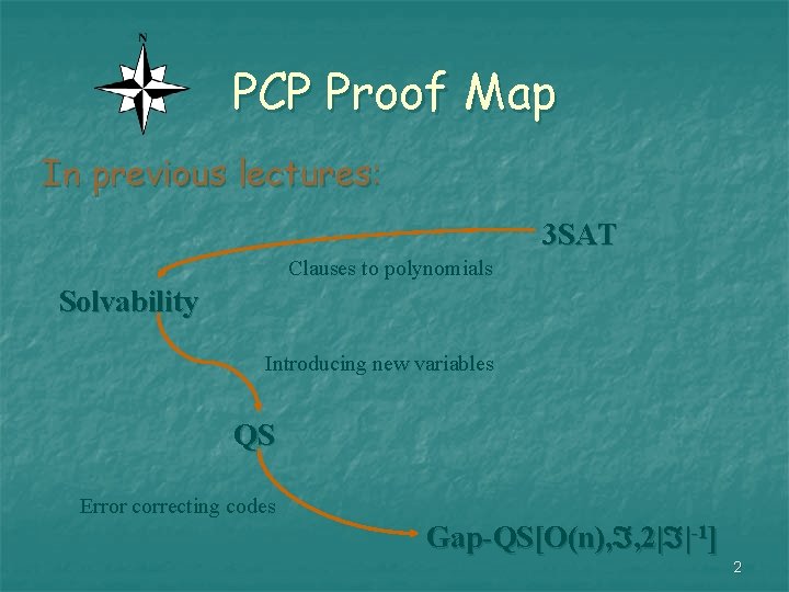
PCP Proof Map In previous lectures: 3 SAT Clauses to polynomials Solvability Introducing new variables QS Error correcting codes Gap-QS[O(n), , 2| |-1] 2

PCP Proof Map Later: Gap-QS[O(n), , 2| |-1] Sum Check quadratic equations of constant size with consistency assumptions Gap-QScons[O(1), , 2| |-1] Consistent Reader Gap-QS*[O(1), , | |- ] Error correcting codes conjunctions of constant number of quadratic equations, whose dependencies are constant. Gap-QS[O(1), , 2| |-1] 3

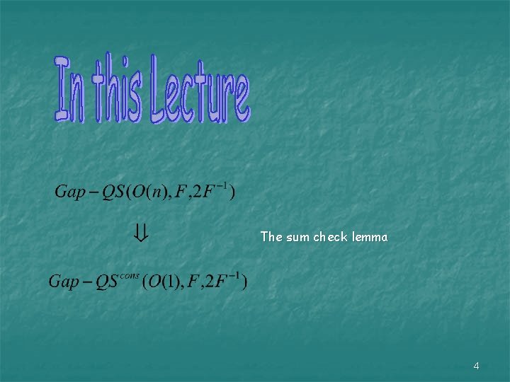
The sum check lemma 4

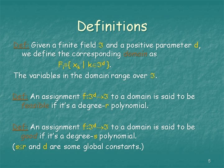
Definitions Def: Given a finite field and a positive parameter d, we define the corresponding domain as Fi={ xk | k d }. The variables in the domain range over . Def: An assignment f: d to a domain is said to be feasible if it’s a degree-r polynomial. Def: An assignment f: d to a domain is said to be good if it’s a degree-s polynomial. (s r and d are some global constants. ) 5

Definitions Def: (Gap-QScons[D, , ]) Instance: A set of domains F 1, . . . , Fk and n quadratic equations over . Each equation depends on at most D variables, some of them belong to certain domains. Problem: to distinguish between: There is a good assignment satisfying all the equations. No more than an fraction of the equations can be satisfied simultaneously by a feasible assignment. 6

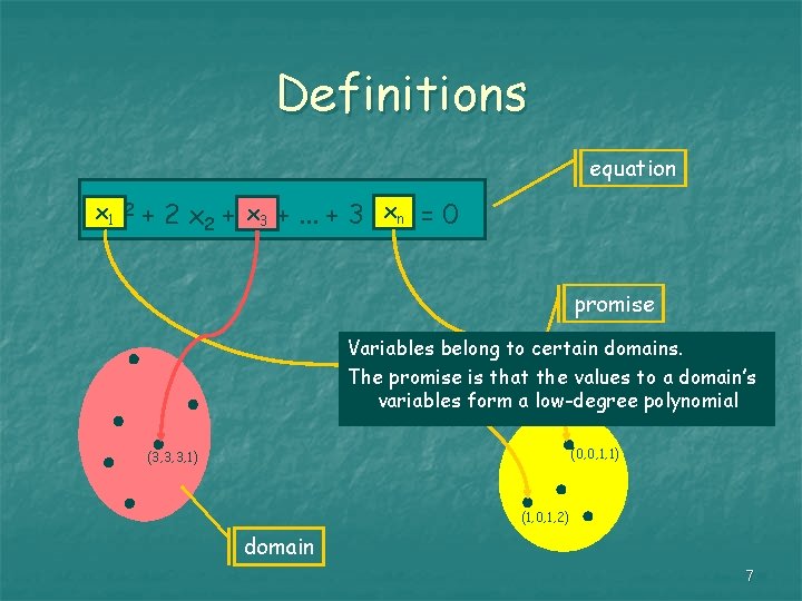
Definitions equation x x 11 2 + 2 x 2 + xx 33 +. . . + 3 xxnn = 0 promise Variables belong to certain domains. The promise is that the values to a domain’s variables form a low-degree polynomial (0, 0, 1, 1) (3, 3, 3, 1) (1, 0, 1, 2) domain 7

The Sum-Check Lemma (Sum-Check): Gap-QS[O(n), , 2/| |] is efficiently reducible to Gap-QScons[O(1), , 2/| |]. 8

Overview We precede the proof by a general scheme: n Our starting point is the gap-QS instance, and we need to decrease (to constant) the number of variables each quadratic-polynomial depends on n We will add variables to those of the original gap. QS instance, to check consistency, and replace each polynomial with many new ones n The consistency will be checked later on in the proof (chapter 2) utilizing the efficient consistent -readers we have seen n Our test assumes the values for some preset sets of variables to correspond to the point-evaluation of a low-degree polynomial (an assumption to be removed by plugging in the consistent reader) 9

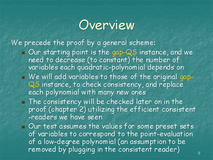
Representing a Quadratic-Polynomial Given a quadratic-polynomial P, over variables Yi, let us write the value of P in a certain point in the space as follows: A is an ( (i, j) is the coefficient of the monomial yiyj ) assignment to the variables Let us convert the polynomial to linear form: let’s assume a set of variables yij, i, j [1. . m], with the intention that A(yij) = A(yi) · A(yj), and the special case where A(yii) = A(yi) which lets us write: 10

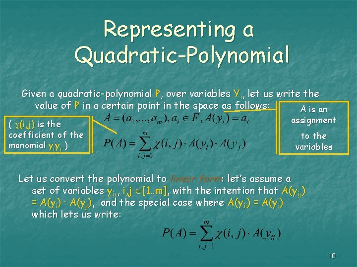
Representing a Quadratic-Polynomial Next, we associate each variable yij with some point x Hd. Define the following one-to-one function: Notice that: As a consequence we can define: For a value in x Hd without a source define: 11

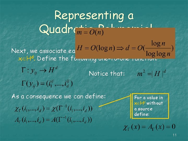
Representing a Quadratic-Polynomial Using the new definitions we can write: Where , A are functions: 12

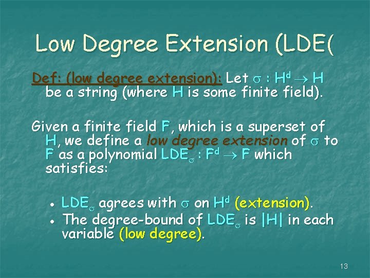
Low Degree Extension (LDE( Def: (low degree extension): Let : Hd H be a string (where H is some finite field). Given a finite field F, which is a superset of H, we define a low degree extension of to F as a polynomial LDE : Fd F which satisfies: · · LDE agrees with on Hd (extension). The degree-bound of LDE is |H| in each variable (low degree). 13

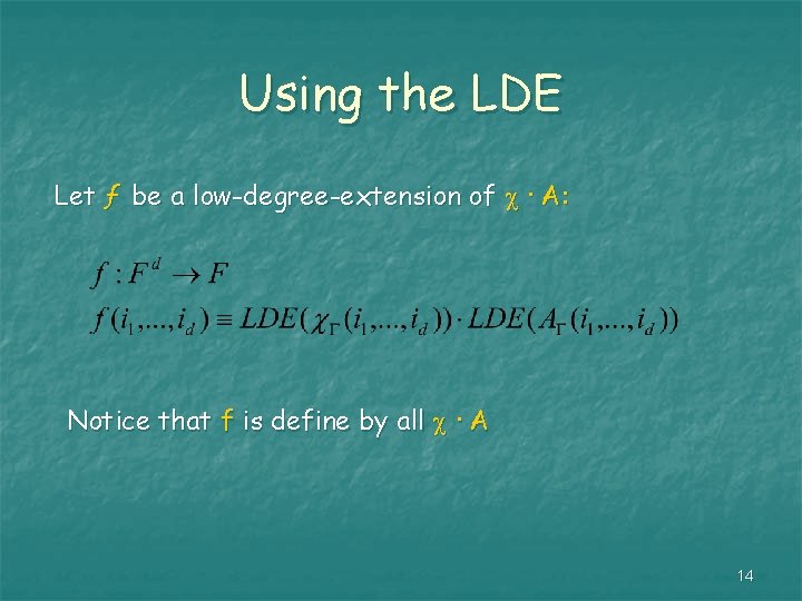
Using the LDE Let ƒ be a low-degree-extension of · A: Notice that f is define by all · A 14

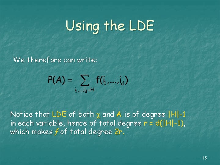
Using the LDE We therefore can write: Notice that LDE of both and A is of degree |H|-1 in each variable, hence of total degree r = d(|H|-1), which makes ƒ of total degree 2 r. 15

What’s ahead We show next a test that uses a small number of variables: For any assignment for which some variables corresponds to a function ƒ of degree 2 r, the test verifies the sum of values of ƒ over Hd equals a given value. Each local-test accesses much smaller number than |Hd| of representation variables. Later on we will replace the assumption that ƒ is a lowdegree-function by evaluating that single point accessed with an efficient consistent-reader for ƒ 16

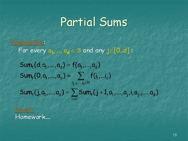
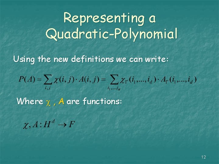
Partial Sums For any j [0. . d] define: That is, Sumƒ is the function that does not vary on the first j variables, and sums over all points for which the rest of the variables are all in H Proposition: Sumƒ is of degree 2 rd Proof: Immediate since ƒ is of degree 2 r and Sumƒ is the linear combination of d degree-r functions 17

Partial Sums Proposition: For every a 1, . . , ad any j [0. . d] : Proof: Homework. . . 18

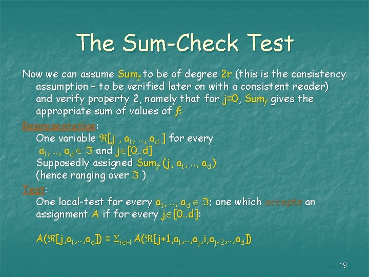
The Sum-Check Test Now we can assume Sumƒ to be of degree 2 r (this is the consistency assumption – to be verified later on with a consistent reader) and verify property 2, namely that for j=0, Sumƒ gives the appropriate sum of values of ƒ: Representation: One variable [j , a 1, . . , ad ] for every a 1, . . , ad and j [0. . d] Supposedly assigned Sumƒ (j, a 1, . . , ad ) (hence ranging over ) Test: One local-test for every a 1, . . , ad ; one which accepts an assignment A if for every j [0. . d]: A( [j, a 1, . . , ad]) = i H A( [j+1, a 1, . . , aj, i, aj+2, . . , ad]) 19

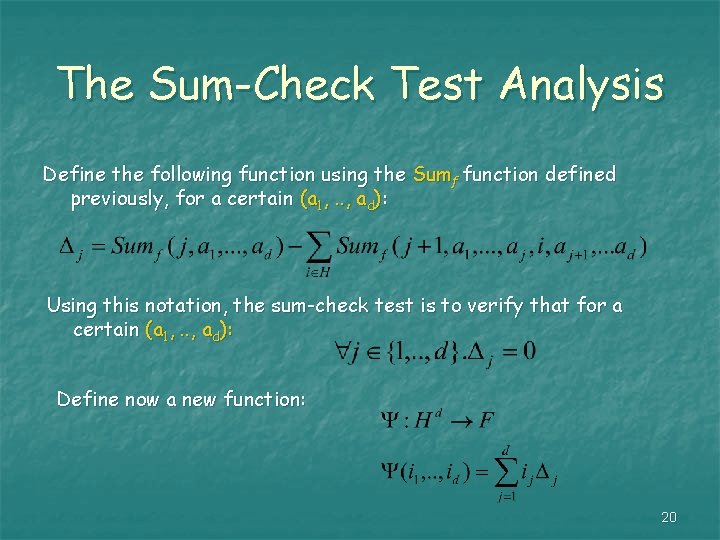
The Sum-Check Test Analysis Define the following function using the Sumƒ function defined previously, for a certain (a 1, . . , ad): Using this notation, the sum-check test is to verify that for a certain (a 1, . . , ad): Define now a new function: 20

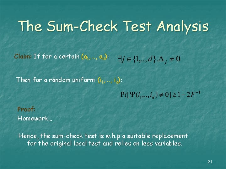
The Sum-Check Test Analysis Claim: If for a certain (a 1, . . , ad): Then for a random uniform (i 1, . . , id): Proof: Homework… Hence, the sum-check test is w. h. p a suitable replacement for the original local test and relies on less variables. 21

The Sum-Check Test Analysis n n n The above test already reduces the number of variables each local test accesses from O(Hd) to O(d |H|). However, we have introduces a consistency assumption (that the functions f are low degree) We shall now reduce the number of variables accessed to a constant O(1) (and strengthen the consistency assumption on the way) using the exact same method. 22

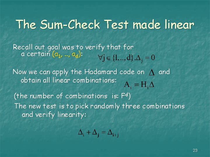
The Sum-Check Test made linear Recall out goal was to verify that for a certain (a 1, . . , ad): Now we can apply the Hadamard code on obtain all linear combinations: and (the number of combinations is: Fd) The new test is to pick randomly three combinations and verify linearity: 23

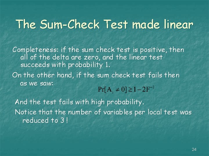
The Sum-Check Test made linear Completeness: if the sum check test is positive, then all of the delta are zero, and the linear test succeeds with probability 1. On the other hand, if the sum check test fails then as we saw: And the test fails with high probability. Notice that the number of variables per local test was reduced to 3 ! 24