1 PCP Proof Map In previous lectures 3

1

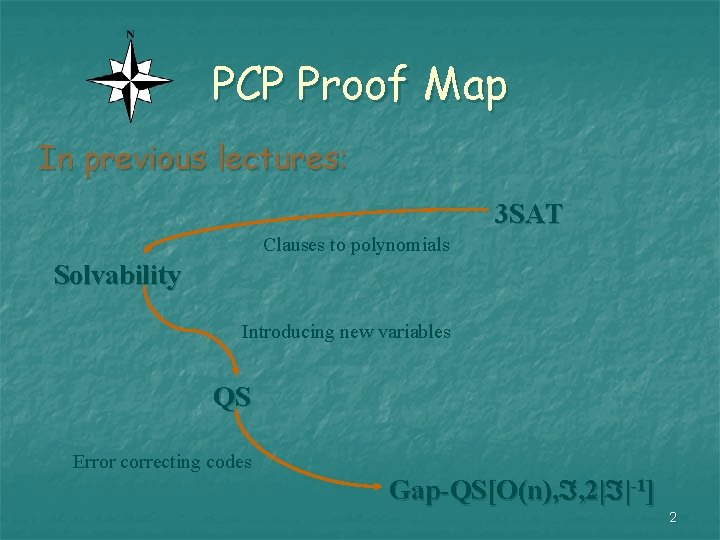
PCP Proof Map In previous lectures: 3 SAT Clauses to polynomials Solvability Introducing new variables QS Error correcting codes Gap-QS[O(n), , 2| |-1] 2

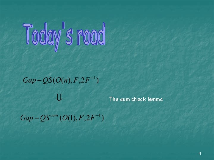
PCP Proof Map In following lectures: Gap-QS[O(n), , 2| |-1] Sum Check quadratic equations of constant size with consistency assumptions Gap-QScons[O(1), , 2| |-1] Consistent Reader Gap-QS*[O(1), , | |- ] Error correcting codes conjunctions of constant number of quadratic equations, whose dependencies are constant. Gap-QS[O(1), , 2| |-1] 3

The sum check lemma 4

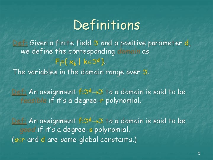
Definitions Def: Given a finite field and a positive parameter d, we define the corresponding domain as Fi={ xk | k d }. The variables in the domain range over . Def: An assignment f: d to a domain is said to be feasible if it’s a degree-r polynomial. Def: An assignment f: d to a domain is said to be good if it’s a degree-s polynomial. (s r and d are some global constants. ) 5

Definitions Def: (Gap-QScons[D, , ]) Instance: A set of domains F 1, . . . , Fk and n quadratic equations over . Each equation depends on at most D variables, some of them belong to some domains. Problem: to distinguish between: There is a good assignment satisfying all the equations. No more than an fraction of the equations can be satisfied simultaneously by a feasible assignment. 6

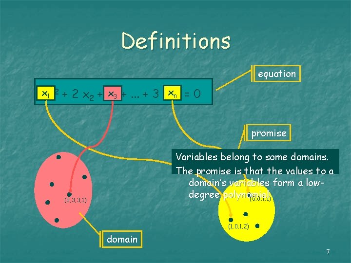
Definitions equation x x 11 2 + 2 x 2 + xx 33 +. . . + 3 xxnn = 0 promise Variables belong to some domains. The promise is that the values to a domain’s variables form a lowdegree polynomial (0, 0, 1, 1) (3, 3, 3, 1) (1, 0, 1, 2) domain 7

The Sum-Check Lemma (Sum-Check): Gap-QS[O(n), , 2/| |] is efficiently reducible to Gap-QScons[O(1), , 2/| |]. 8

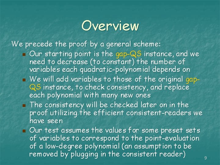
Overview We precede the proof by a general scheme: n Our starting point is the gap-QS instance, and we need to decrease (to constant) the number of variables each quadratic-polynomial depends on n We will add variables to those of the original gap. QS instance, to check consistency, and replace each polynomial with many new ones n The consistency will be checked later on in the proof utilizing the efficient consistent-readers we have seen n Our test assumes the values for some preset sets of variables to correspond to the point-evaluation of a low-degree polynomial (an assumption to be removed by plugging in the consistent reader) 9

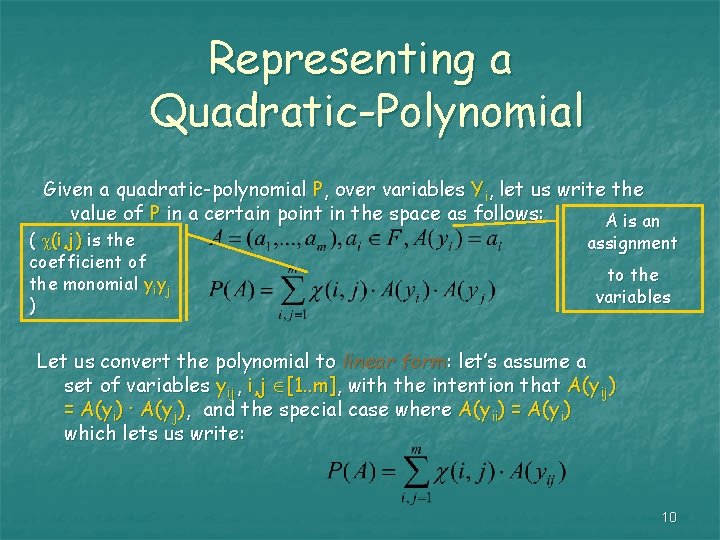
Representing a Quadratic-Polynomial Given a quadratic-polynomial P, over variables Yi, let us write the value of P in a certain point in the space as follows: A is an ( (i, j) is the coefficient of the monomial yiyj ) assignment to the variables Let us convert the polynomial to linear form: let’s assume a set of variables yij, i, j [1. . m], with the intention that A(yij) = A(yi) · A(yj), and the special case where A(yii) = A(yi) which lets us write: 10

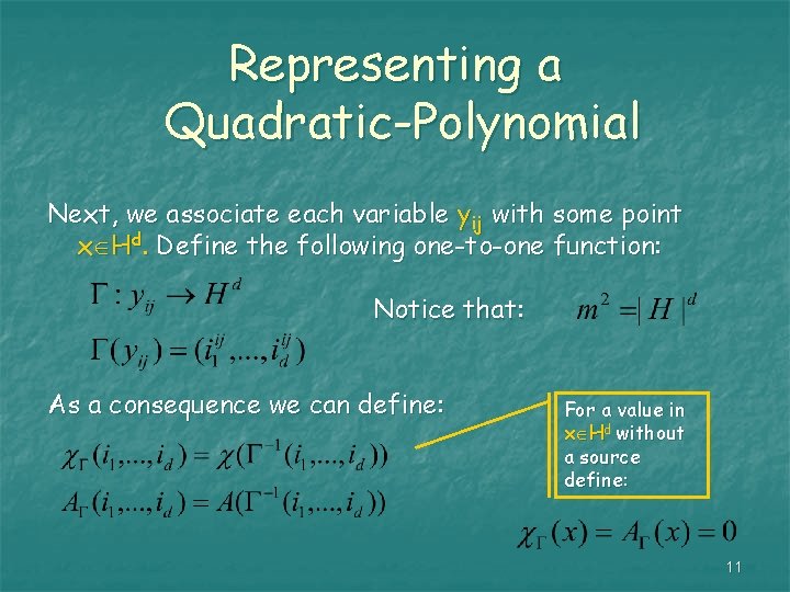
Representing a Quadratic-Polynomial Next, we associate each variable yij with some point x Hd. Define the following one-to-one function: Notice that: As a consequence we can define: For a value in x Hd without a source define: 11

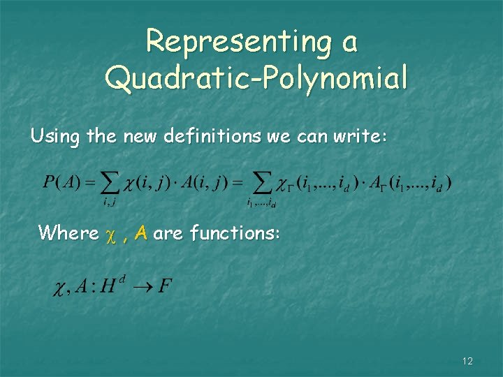
Representing a Quadratic-Polynomial Using the new definitions we can write: Where , A are functions: 12

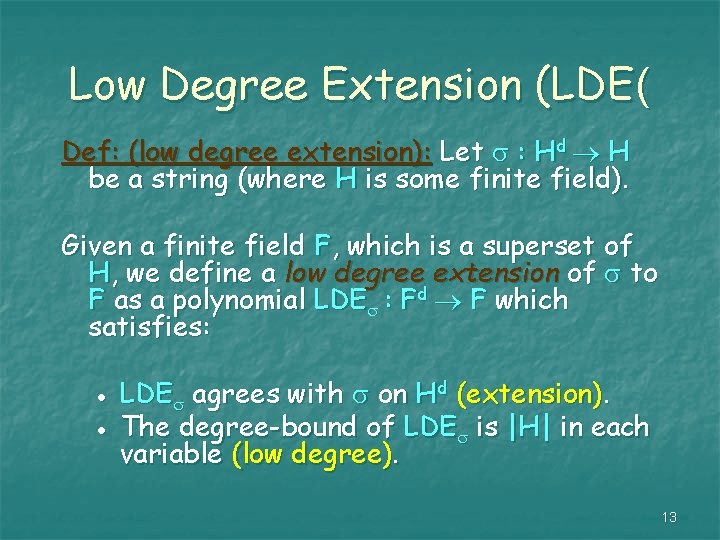
Low Degree Extension (LDE( Def: (low degree extension): Let : Hd H be a string (where H is some finite field). Given a finite field F, which is a superset of H, we define a low degree extension of to F as a polynomial LDE : Fd F which satisfies: · · LDE agrees with on Hd (extension). The degree-bound of LDE is |H| in each variable (low degree). 13

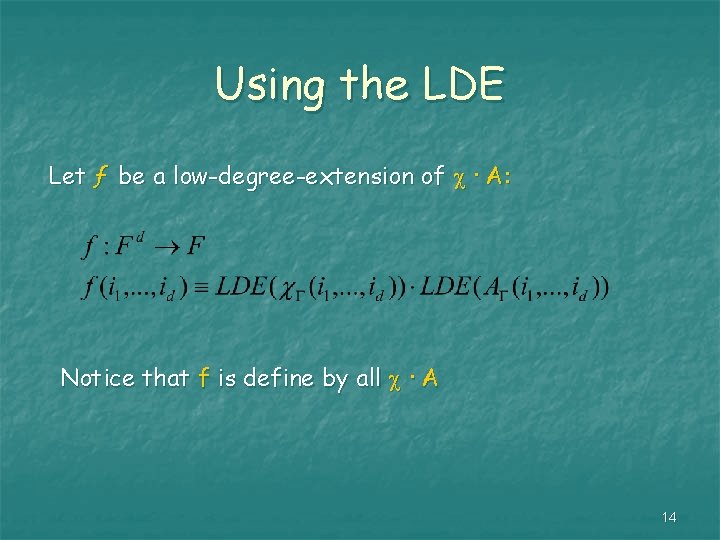
Using the LDE Let ƒ be a low-degree-extension of · A: Notice that f is define by all · A 14

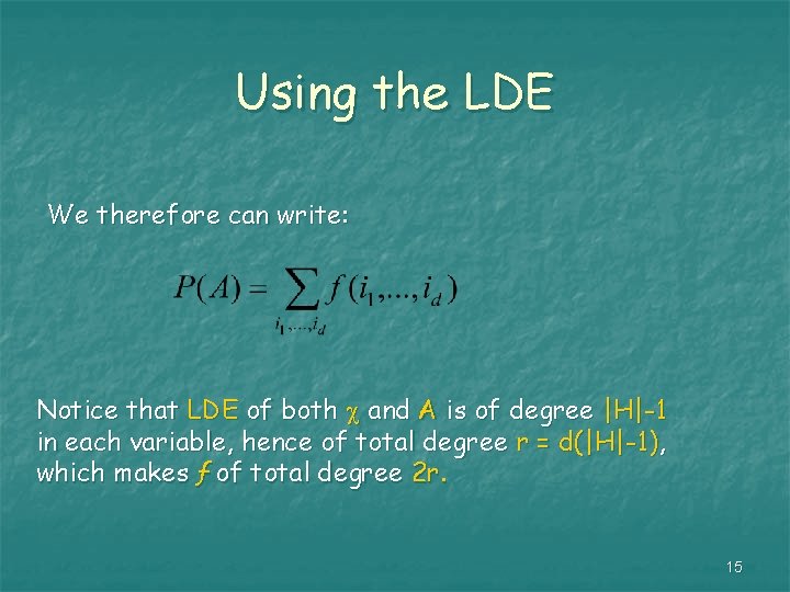
Using the LDE We therefore can write: Notice that LDE of both and A is of degree |H|-1 in each variable, hence of total degree r = d(|H|-1), which makes ƒ of total degree 2 r. 15

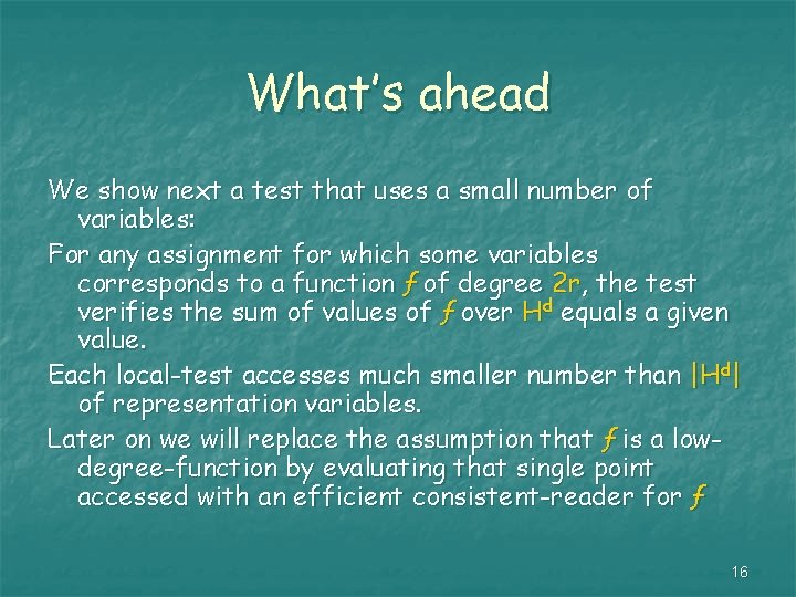
What’s ahead We show next a test that uses a small number of variables: For any assignment for which some variables corresponds to a function ƒ of degree 2 r, the test verifies the sum of values of ƒ over Hd equals a given value. Each local-test accesses much smaller number than |Hd| of representation variables. Later on we will replace the assumption that ƒ is a lowdegree-function by evaluating that single point accessed with an efficient consistent-reader for ƒ 16

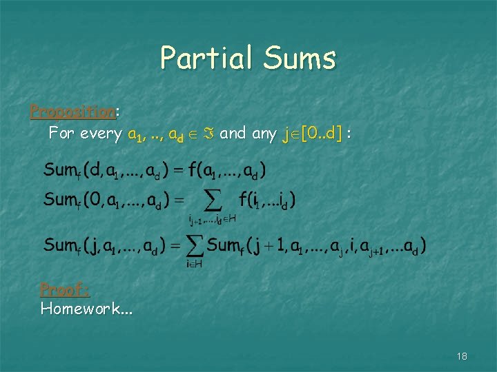
Partial Sums For any j [0. . d] define: That is, Sumƒ is the function that does not vary on the first j variables, and sums over all points for which the rest of the variables are all in H Proposition: Sumƒ is of degree 2 rd Proof: Immediate since ƒ is of degree 2 r and Sumƒ is the linear combination of d degree-r functions 17

Partial Sums Proposition: For every a 1, . . , ad any j [0. . d] : Proof: Homework. . . 18

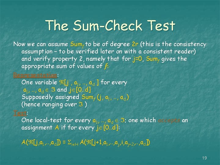
The Sum-Check Test Now we can assume Sumƒ to be of degree 2 r (this is the consistency assumption – to be verified later on with a consistent reader) and verify property 2, namely that for j=0, Sumƒ gives the appropriate sum of values of ƒ: Representation: One variable [j , a 1, . . , ad ] for every a 1, . . , ad and j [0. . d] Supposedly assigned Sumƒ (j, a 1, . . , ad ) (hence ranging over ) Test: One local-test for every a 1, . . , ad ; one which accepts an assignment A if for every j [0. . d]: A( [j, a 1, . . , ad]) = i H A( [j+1, a 1, . . , aj, i, aj+2, . . , ad]) 19

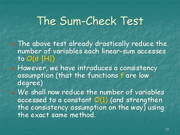
The Sum-Check Test n n n The above test already drastically reduce the number of variables each linear-sum accesses to O(d |H|) However, we have introduces a consistency assumption (that the functions f are low degree) We shall now reduce the number of variables accessed to a constant O(1) (and strengthen the consistency assumption on the way) using the exact same method. 20

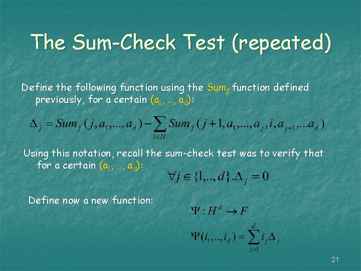
The Sum-Check Test (repeated) Define the following function using the Sumƒ function defined previously, for a certain (a 1, . . , ad): Using this notation, recall the sum-check test was to verify that for a certain (a 1, . . , ad): Define now a new function: 21

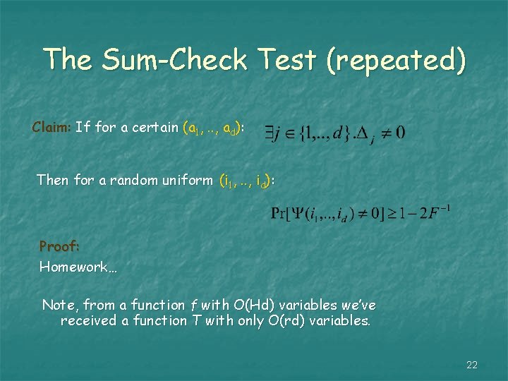
The Sum-Check Test (repeated) Claim: If for a certain (a 1, . . , ad): Then for a random uniform (i 1, . . , id): Proof: Homework… Note, from a function f with O(Hd) variables we’ve received a function T with only O(rd) variables. 22

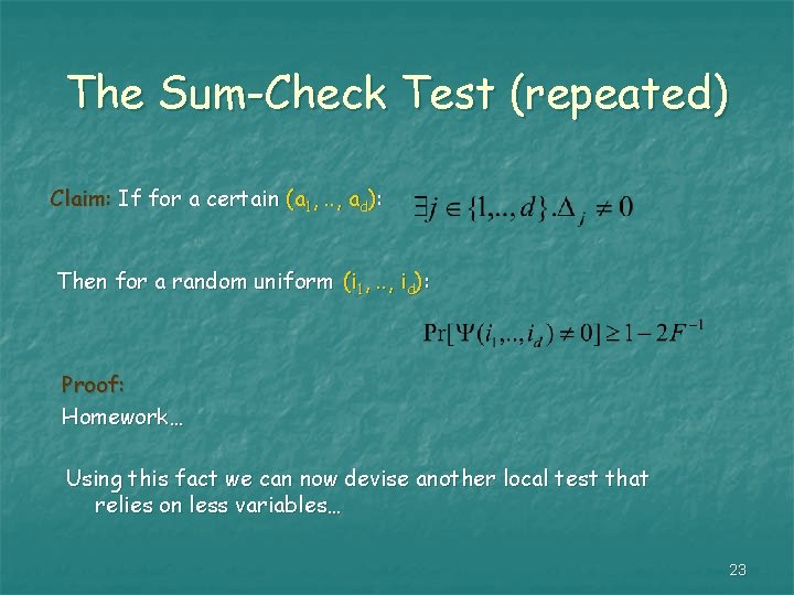
The Sum-Check Test (repeated) Claim: If for a certain (a 1, . . , ad): Then for a random uniform (i 1, . . , id): Proof: Homework… Using this fact we can now devise another local test that relies on less variables… 23