0 Introduction to Game Theory Lirong Xia Voting

0

Introduction to Game Theory Lirong Xia

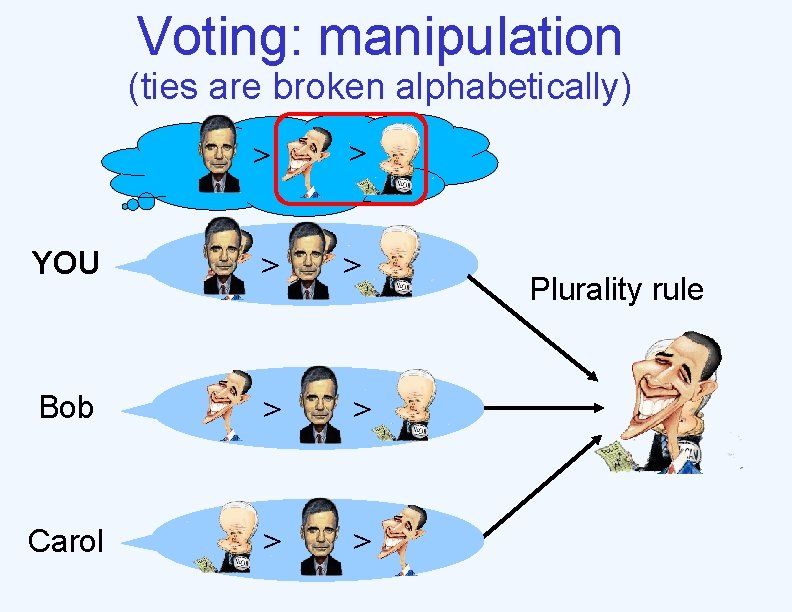
Voting: manipulation (ties are broken alphabetically) > > YOU > > Bob > > Carol > > Plurality rule

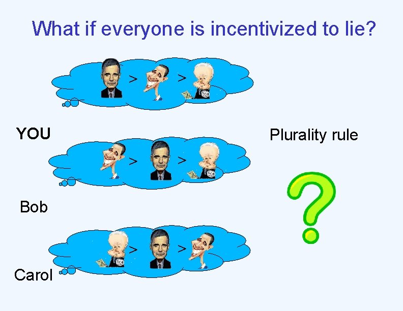
What if everyone is incentivized to lie? > > YOU Plurality rule > > Bob Carol

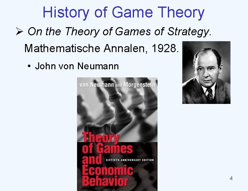
History of Game Theory Ø On the Theory of Games of Strategy. Mathematische Annalen, 1928. • John von Neumann 4

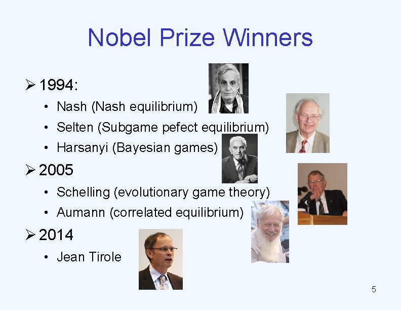
Nobel Prize Winners Ø 1994: • Nash (Nash equilibrium) • Selten (Subgame pefect equilibrium) • Harsanyi (Bayesian games) Ø 2005 • Schelling (evolutionary game theory) • Aumann (correlated equilibrium) Ø 2014 • Jean Tirole 5

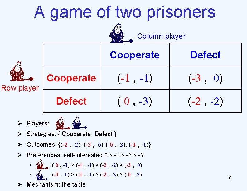
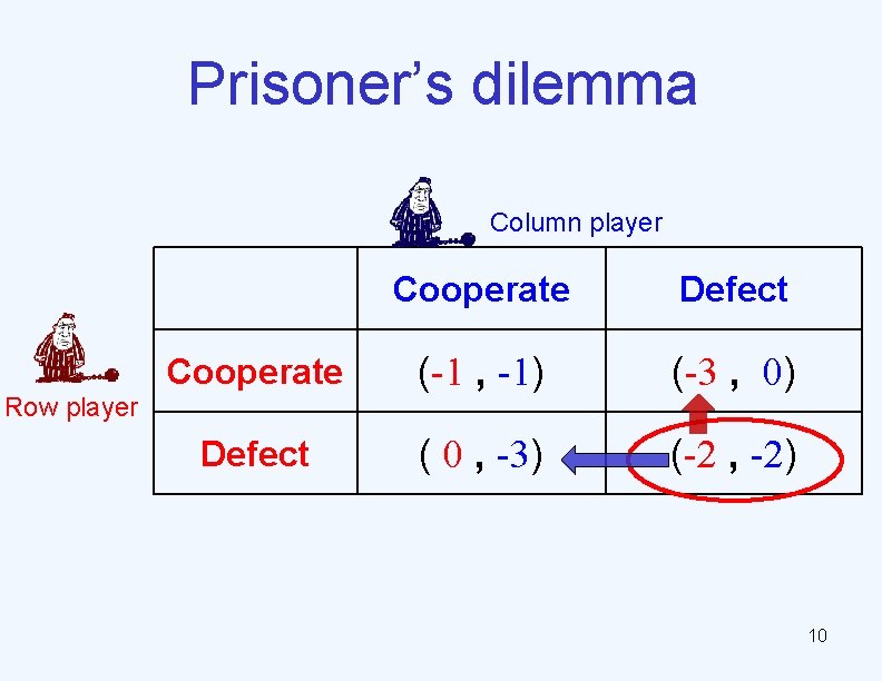
A game of two prisoners Column player Cooperate Defect Cooperate (-1 , -1) (-3 , 0) Defect ( 0 , -3) (-2 , -2) Row player Ø Players: Ø Strategies: { Cooperate, Defect } Ø Outcomes: {(-2 , -2), (-3 , 0), ( 0 , -3), (-1 , -1)} Ø Preferences: self-interested 0 > -1 > -2 > -3 • : ( 0 , -3) > (-1 , -1) > (-2 , -2) > (-3 , 0) • : (-3 , 0) > (-1 , -1) > (-2 , -2) > ( 0 , -3) Ø Mechanism: the table 6

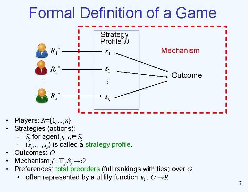
Formal Definition of a Game R 1* Strategy Profile D s 1 s 2 R n* sn … … R 2* Mechanism Outcome • Players: N={1, …, n} • Strategies (actions): - Sj for agent j, sj∈Sj - (s 1, …, sn) is called a strategy profile. • Outcomes: O • Mechanism f : Πj Sj →O • Preferences: total preorders (full rankings with ties) over O • often represented by a utility function ui : O →R 7

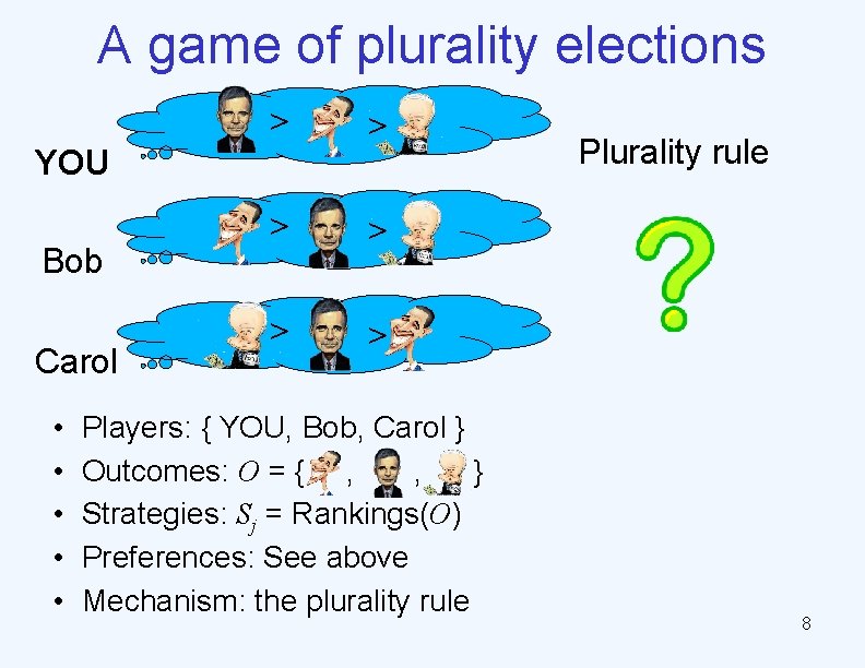
A game of plurality elections > > > YOU Bob Carol • • • Players: { YOU, Bob, Carol } Outcomes: O = { , , } Strategies: Sj = Rankings(O) Preferences: See above Mechanism: the plurality rule Plurality rule 8

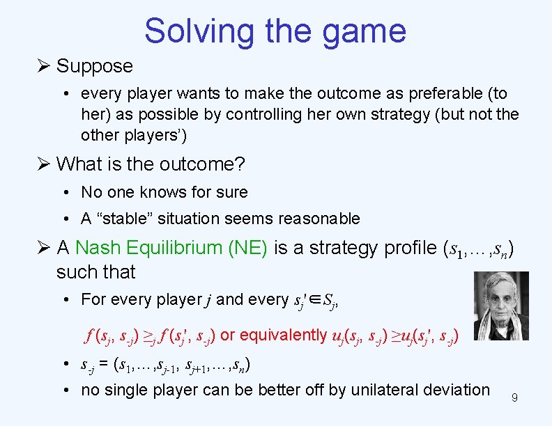
Solving the game Ø Suppose • every player wants to make the outcome as preferable (to her) as possible by controlling her own strategy (but not the other players’) Ø What is the outcome? • No one knows for sure • A “stable” situation seems reasonable Ø A Nash Equilibrium (NE) is a strategy profile (s 1, …, sn) such that • For every player j and every sj'∈Sj, f (sj, s-j) ≥j f (sj', s-j) or equivalently uj(sj, s-j) ≥uj(sj', s-j) • s-j = (s 1, …, sj-1, sj+1, …, sn) • no single player can be better off by unilateral deviation 9

Prisoner’s dilemma Column player Cooperate Defect Cooperate (-1 , -1) (-3 , 0) Defect ( 0 , -3) (-2 , -2) Row player 10

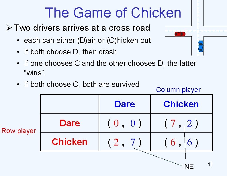
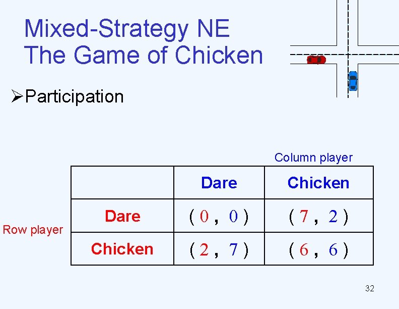
The Game of Chicken Ø Two drivers arrives at a cross road • each can either (D)air or (C)hicken out • If both choose D, then crash. • If one chooses C and the other chooses D, the latter “wins”. • If both choose C, both are survived Row player Column player Dare Chicken Dare (0, 0) (7, 2) Chicken (2, 7) (6, 6) NE 11

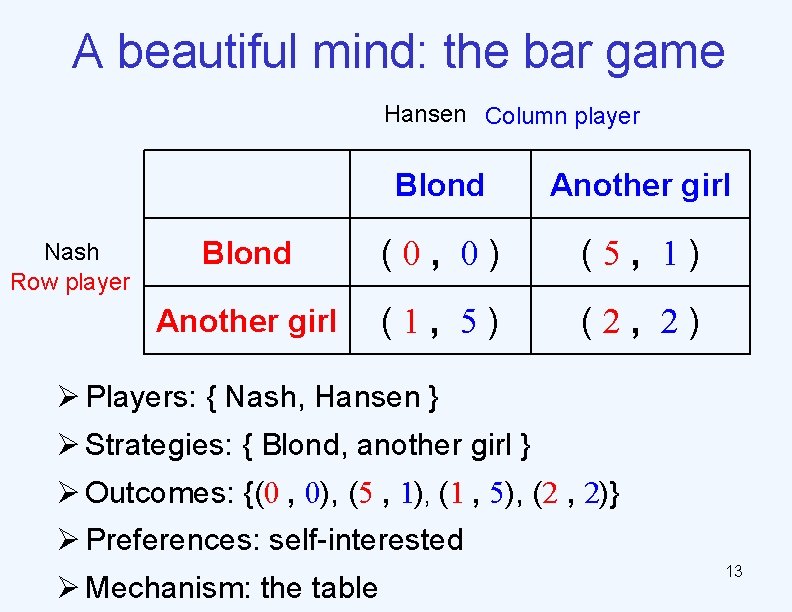
A beautiful mind Ø “If everyone competes for the blond, we block each other and no one gets her. So then we all go for her friends. But they give us the cold shoulder, because no one likes to be second choice. Again, no winner. But what if none of us go for the blond. We don’t get in each other’s way, we don’t insult the other girls. That’s the only way we win. That’s the only way we all get [a girl. ]” 12

A beautiful mind: the bar game Hansen Column player Nash Row player Blond Another girl Blond (0, 0) (5, 1) Another girl (1, 5) (2, 2) Ø Players: { Nash, Hansen } Ø Strategies: { Blond, another girl } Ø Outcomes: {(0 , 0), (5 , 1), (1 , 5), (2 , 2)} Ø Preferences: self-interested Ø Mechanism: the table 13

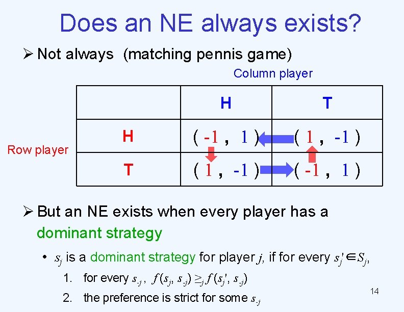
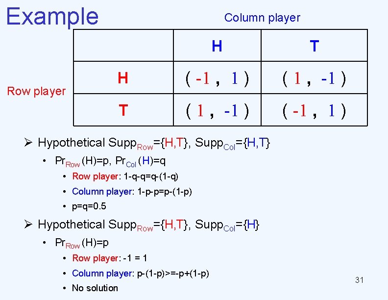
Does an NE always exists? Ø Not always (matching pennis game) Column player Row player H T H ( -1 , 1 ) ( 1 , -1 ) T ( 1 , -1 ) ( -1 , 1 ) Ø But an NE exists when every player has a dominant strategy • sj is a dominant strategy for player j, if for every sj'∈Sj, 1. for every s-j , f (sj, s-j) ≥j f (sj', s-j) 2. the preference is strict for some s-j 14

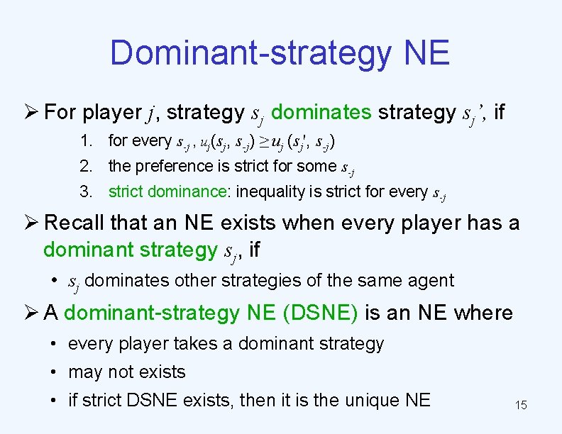
Dominant-strategy NE Ø For player j, strategy sj dominates strategy sj’, if 1. for every s-j , uj(sj, s-j) ≥ uj (sj', s-j) 2. the preference is strict for some s-j 3. strict dominance: inequality is strict for every s-j Ø Recall that an NE exists when every player has a dominant strategy sj, if • sj dominates other strategies of the same agent Ø A dominant-strategy NE (DSNE) is an NE where • every player takes a dominant strategy • may not exists • if strict DSNE exists, then it is the unique NE 15

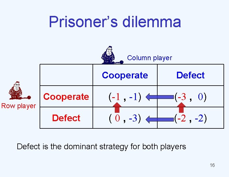
Prisoner’s dilemma Column player Cooperate Defect Cooperate (-1 , -1) (-3 , 0) Defect ( 0 , -3) (-2 , -2) Row player Defect is the dominant strategy for both players 16

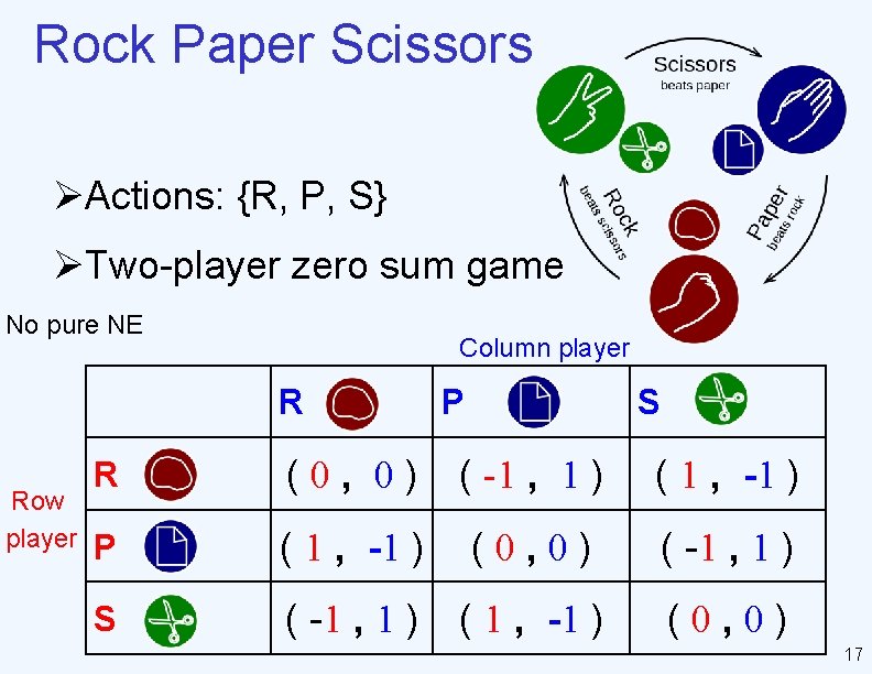
Rock Paper Scissors ØActions: {R, P, S} ØTwo-player zero sum game No pure NE Column player R Row player P S R (0, 0) ( -1 , 1 ) ( 1 , -1 ) P ( 1 , -1 ) (0, 0) ( -1 , 1 ) S ( -1 , 1 ) ( 1 , -1 ) (0, 0) 17

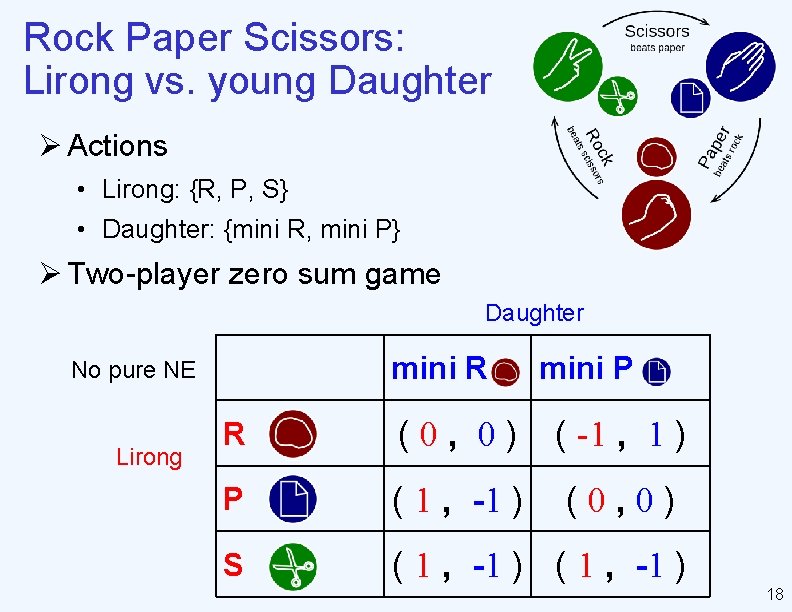
Rock Paper Scissors: Lirong vs. young Daughter Ø Actions • Lirong: {R, P, S} • Daughter: {mini R, mini P} Ø Two-player zero sum game Daughter mini R No pure NE Lirong mini P R (0, 0) ( -1 , 1 ) P ( 1 , -1 ) (0, 0) S ( 1 , -1 ) 18

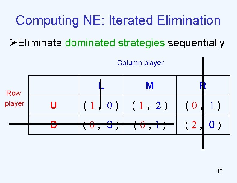
Computing NE: Iterated Elimination ØEliminate dominated strategies sequentially Column player Row player L M R U (1, 0) (1, 2) (0, 1) D (0, 3) (0, 1) (2, 0) 19

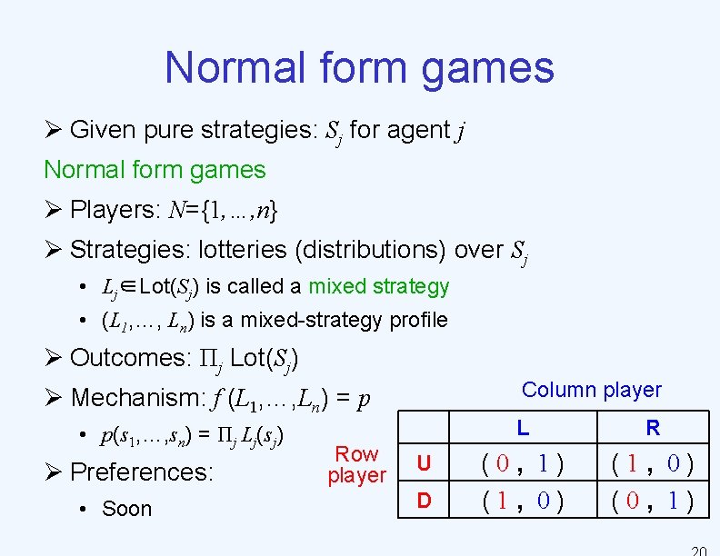
Normal form games Ø Given pure strategies: Sj for agent j Normal form games Ø Players: N={1, …, n} Ø Strategies: lotteries (distributions) over Sj • Lj∈Lot(Sj) is called a mixed strategy • (L 1, …, Ln) is a mixed-strategy profile Ø Outcomes: Πj Lot(Sj) Column player Ø Mechanism: f (L 1, …, Ln) = p • p(s 1, …, sn) = Πj Lj(sj) Ø Preferences: • Soon Row player U D L R (0, 1) (1, 0) (0, 1)

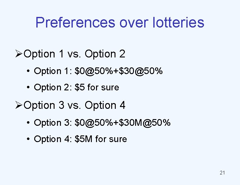
Preferences over lotteries ØOption 1 vs. Option 2 • Option 1: $0@50%+$30@50% • Option 2: $5 for sure ØOption 3 vs. Option 4 • Option 3: $0@50%+$30 M@50% • Option 4: $5 M for sure 21

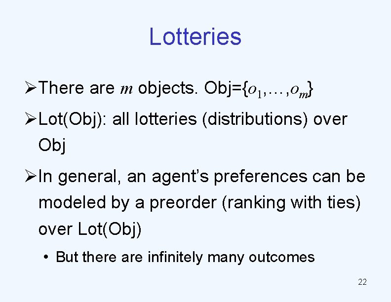
Lotteries ØThere are m objects. Obj={o 1, …, om} ØLot(Obj): all lotteries (distributions) over Obj ØIn general, an agent’s preferences can be modeled by a preorder (ranking with ties) over Lot(Obj) • But there are infinitely many outcomes 22

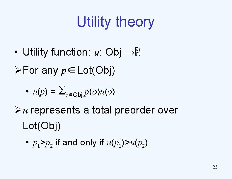
Utility theory • Utility function: u: Obj →ℝ ØFor any p∈Lot(Obj) • u(p) = Σo∈Obj p(o)u(o) Øu represents a total preorder over Lot(Obj) • p 1>p 2 if and only if u(p 1)>u(p 2) 23

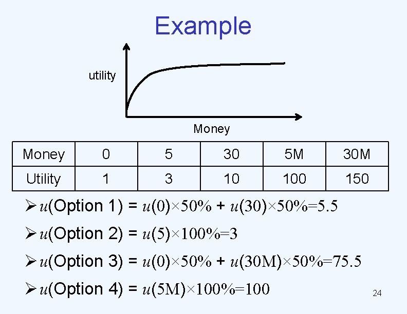
Example utility Money 0 5 30 5 M 30 M Utility 1 3 10 100 150 Ø u(Option 1) = u(0)× 50% + u(30)× 50%=5. 5 Ø u(Option 2) = u(5)× 100%=3 Ø u(Option 3) = u(0)× 50% + u(30 M)× 50%=75. 5 Ø u(Option 4) = u(5 M)× 100%=100 24

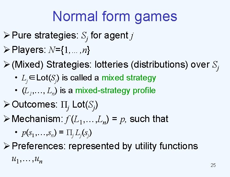
Normal form games Ø Pure strategies: Sj for agent j Ø Players: N={1, …, n} Ø (Mixed) Strategies: lotteries (distributions) over Sj • Lj∈Lot(Sj) is called a mixed strategy • (L 1, …, Ln) is a mixed-strategy profile Ø Outcomes: Πj Lot(Sj) Ø Mechanism: f (L 1, …, Ln) = p, such that • p(s 1, …, sn) = Πj Lj(sj) Ø Preferences: represented by utility functions u 1, …, un 25

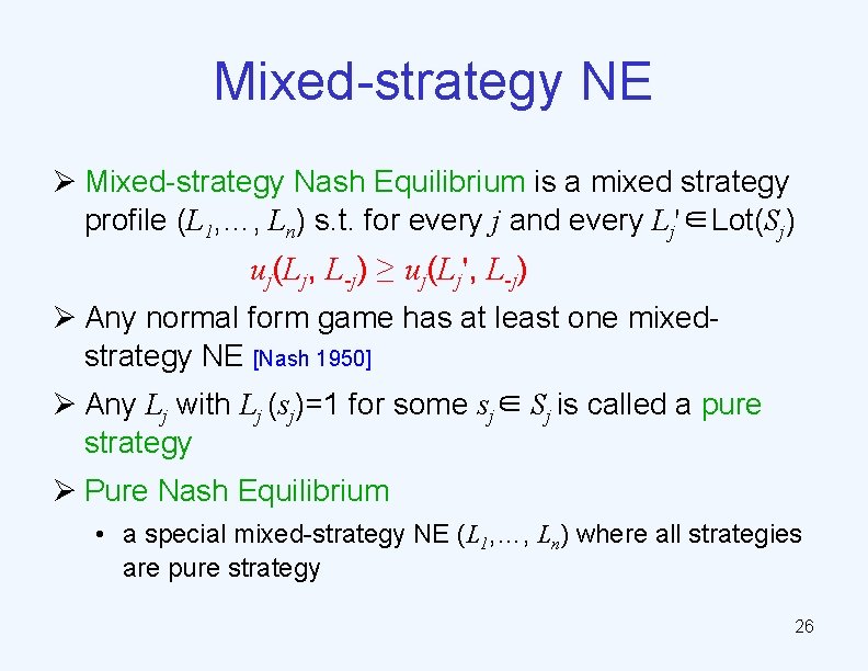
Mixed-strategy NE Ø Mixed-strategy Nash Equilibrium is a mixed strategy profile (L 1, …, Ln) s. t. for every j and every Lj'∈Lot(Sj) uj(Lj, L-j) ≥ uj(Lj', L-j) Ø Any normal form game has at least one mixedstrategy NE [Nash 1950] Ø Any Lj with Lj (sj)=1 for some sj∈ Sj is called a pure strategy Ø Pure Nash Equilibrium • a special mixed-strategy NE (L 1, …, Ln) where all strategies are pure strategy 26

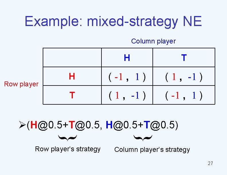
Example: mixed-strategy NE Column player Row player H T H ( -1 , 1 ) ( 1 , -1 ) T ( 1 , -1 ) ( -1 , 1 ) Ø(H@0. 5+T@0. 5, H@0. 5+T@0. 5) } } Row player’s strategy Column player’s strategy 27

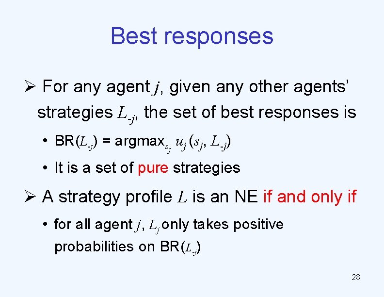
Best responses Ø For any agent j, given any other agents’ strategies L-j, the set of best responses is • BR(L-j) = argmaxsj uj (sj, L-j) • It is a set of pure strategies Ø A strategy profile L is an NE if and only if • for all agent j, Lj only takes positive probabilities on BR(L-j) 28

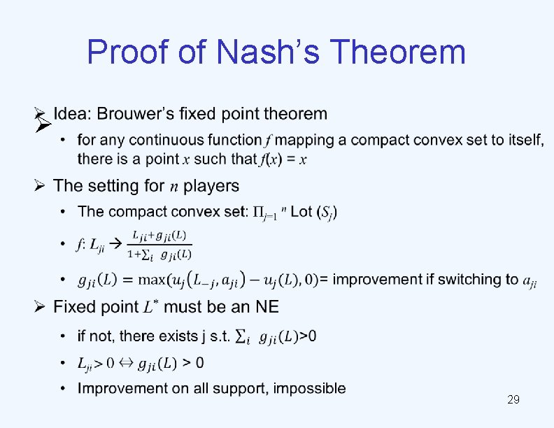
Proof of Nash’s Theorem Ø 29

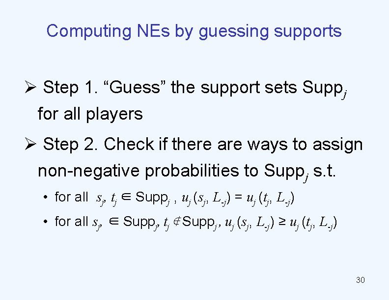
Computing NEs by guessing supports Ø Step 1. “Guess” the support sets Suppj for all players Ø Step 2. Check if there are ways to assign non-negative probabilities to Suppj s. t. • for all sj, tj ∈ Suppj , uj (sj, L-j) = uj (tj, L-j) • for all sj, ∈ Suppj, tj ∉ Suppj , uj (sj, L-j) ≥ uj (tj, L-j) 30

Example Row player Column player H T H ( -1 , 1 ) ( 1 , -1 ) T ( 1 , -1 ) ( -1 , 1 ) Ø Hypothetical Supp. Row={H, T}, Supp. Col={H, T} • Pr. Row (H)=p, Pr. Col (H)=q • Row player: 1 -q-q=q-(1 -q) • Column player: 1 -p-p=p-(1 -p) • p=q=0. 5 Ø Hypothetical Supp. Row={H, T}, Supp. Col={H} • Pr. Row (H)=p • Row player: -1 = 1 • Column player: p-(1 -p)>=-p+(1 -p) • No solution 31

Mixed-Strategy NE The Game of Chicken ØParticipation Column player Row player Dare Chicken Dare (0, 0) (7, 2) Chicken (2, 7) (6, 6) 32

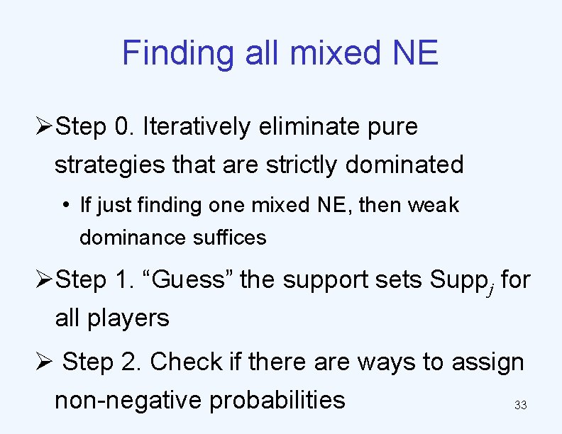
Finding all mixed NE ØStep 0. Iteratively eliminate pure strategies that are strictly dominated • If just finding one mixed NE, then weak dominance suffices ØStep 1. “Guess” the support sets Suppj for all players Ø Step 2. Check if there are ways to assign non-negative probabilities 33

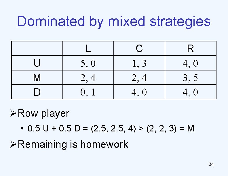
Dominated by mixed strategies U M D L 5, 0 2, 4 0, 1 C 1, 3 2, 4 4, 0 R 4, 0 3, 5 4, 0 ØRow player • 0. 5 U + 0. 5 D = (2. 5, 4) > (2, 2, 3) = M ØRemaining is homework 34

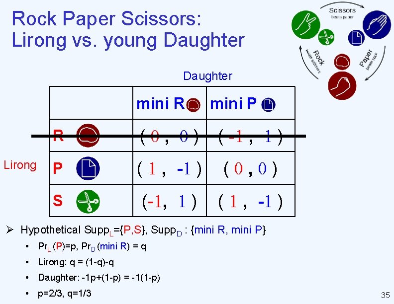
Rock Paper Scissors: Lirong vs. young Daughter mini R Lirong mini P R (0, 0) ( -1 , 1 ) P ( 1 , -1 ) (0, 0) S (-1, 1 ) ( 1 , -1 ) Ø Hypothetical Supp. L={P, S}, Supp. D : {mini R, mini P} • Pr. L (P)=p, Pr. D (mini R) = q • Lirong: q = (1 -q)-q • Daughter: -1 p+(1 -p) = -1(1 -p) • p=2/3, q=1/3 35

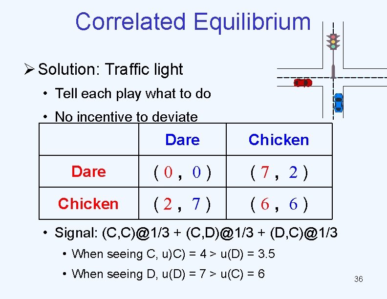
Correlated Equilibrium Ø Solution: Traffic light • Tell each play what to do • No incentive to deviate Dare Chicken Dare (0, 0) (7, 2) Chicken (2, 7) (6, 6) • Signal: (C, C)@1/3 + (C, D)@1/3 + (D, C)@1/3 • When seeing C, u)C) = 4 > u(D) = 3. 5 • When seeing D, u(D) = 7 > u(C) = 6 36

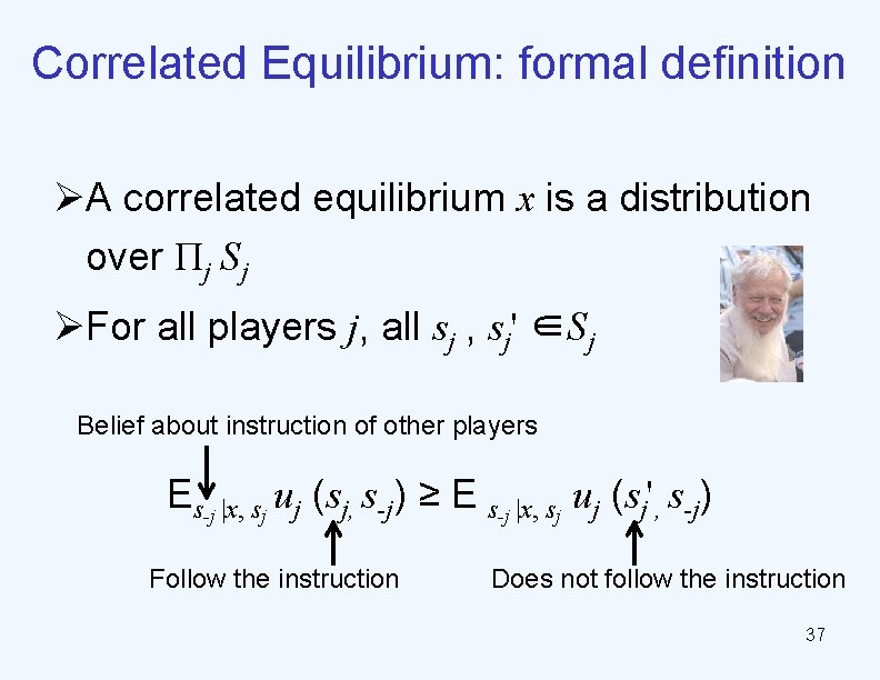
Correlated Equilibrium: formal definition ØA correlated equilibrium x is a distribution over Πj Sj ØFor all players j, all sj , sj' ∈Sj Belief about instruction of other players Es-j |x, sj uj (sj, s-j) ≥ E s-j |x, sj uj (sj', s-j) Follow the instruction Does not follow the instruction 37

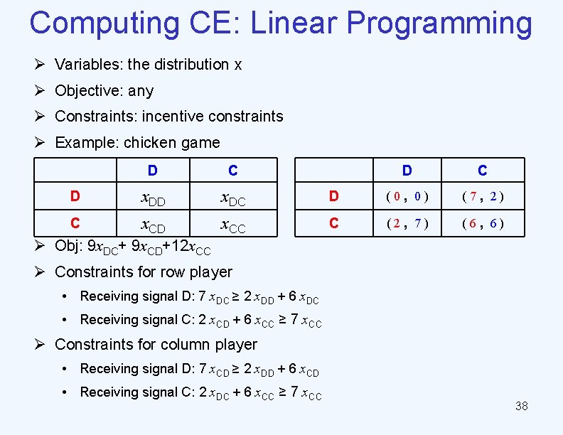
Computing CE: Linear Programming Ø Variables: the distribution x Ø Objective: any Ø Constraints: incentive constraints Ø Example: chicken game D C D x. DC C x. CD x. CC D (0, 0) (7, 2) C (2, 7) (6, 6) Ø Obj: 9 x. DC+ 9 x. CD+12 x. CC Ø Constraints for row player • Receiving signal D: 7 x. DC ≥ 2 x. DD + 6 x. DC • Receiving signal C: 2 x. CD + 6 x. CC ≥ 7 x. CC Ø Constraints for column player • Receiving signal D: 7 x. CD ≥ 2 x. DD + 6 x. CD • Receiving signal C: 2 x. DC + 6 x. CC ≥ 7 x. CC 38

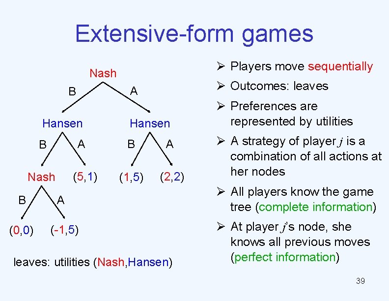
Extensive-form games Ø Players move sequentially Nash B Hansen A B (5, 1) Nash B (0, 0) A Ø Outcomes: leaves Hansen Ø Preferences are represented by utilities B A (1, 5) (2, 2) A (-1, 5) leaves: utilities (Nash, Hansen) Ø A strategy of player j is a combination of all actions at her nodes Ø All players know the game tree (complete information) Ø At player j’s node, she knows all previous moves (perfect information) 39

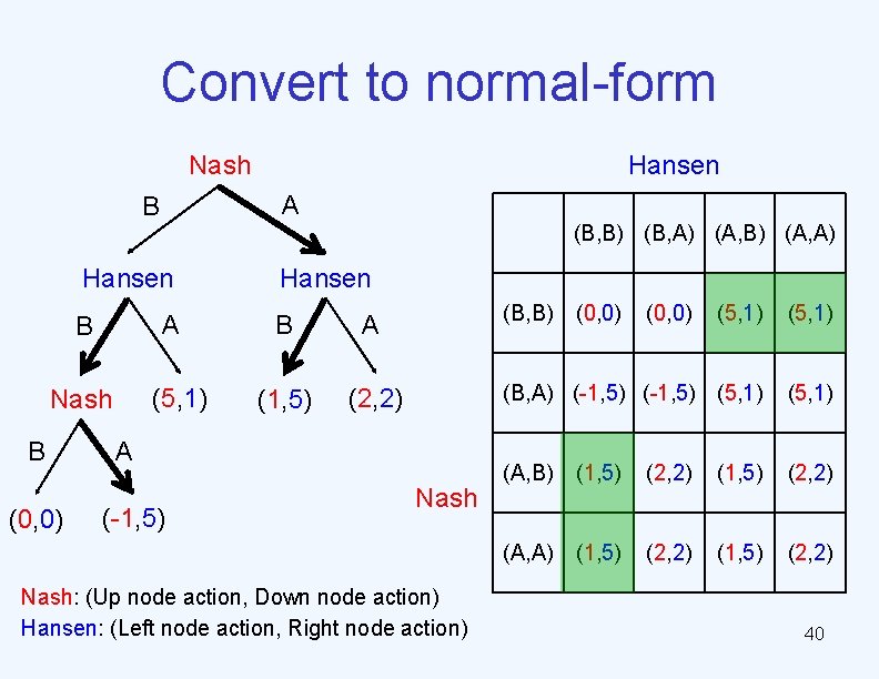
Convert to normal-form Nash A B (B, B) (B, A) (A, B) (A, A) Hansen A B (5, 1) Nash B (0, 0) Hansen B A (1, 5) (2, 2) (B, B) A (-1, 5) Nash: (Up node action, Down node action) Hansen: (Left node action, Right node action) (0, 0) (5, 1) (B, A) (-1, 5) (5, 1) (A, B) (1, 5) (2, 2) (A, A) (1, 5) (2, 2) 40

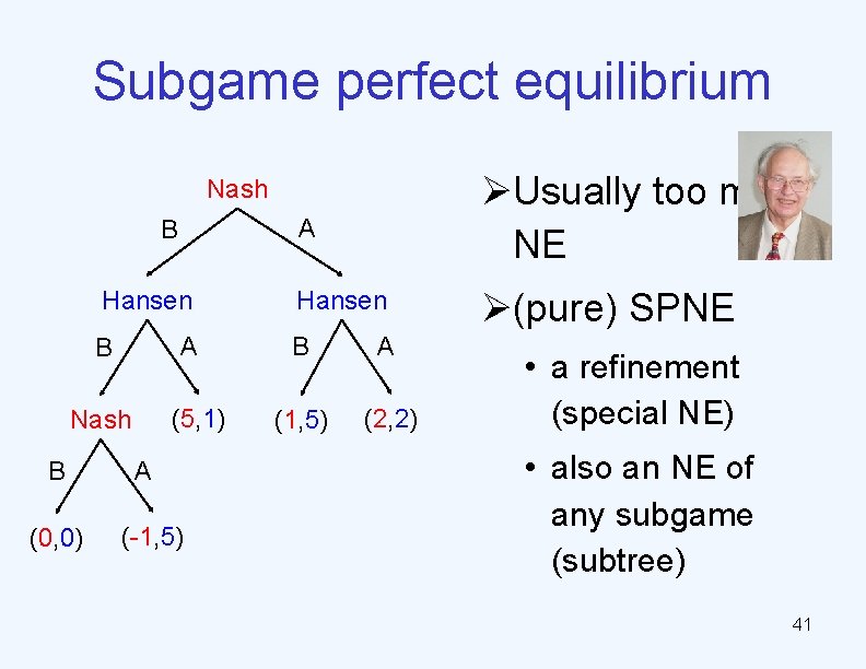
Subgame perfect equilibrium A ØUsually too many NE Hansen Ø(pure) SPNE Nash B Hansen A B (5, 1) Nash B (0, 0) A (-1, 5) B A (1, 5) (2, 2) • a refinement (special NE) • also an NE of any subgame (subtree) 41

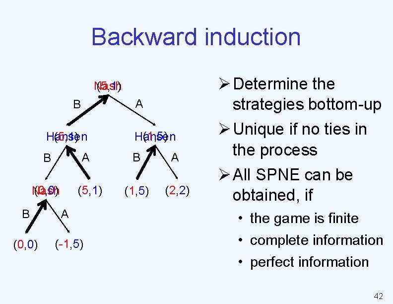
Backward induction Nash (5, 1) A B Hansen (5, 1) A B (0, 0) Nash B (0, 0) (5, 1) A (-1, 5) (1, 5) Hansen B A (1, 5) (2, 2) Ø Determine the strategies bottom-up Ø Unique if no ties in the process Ø All SPNE can be obtained, if • the game is finite • complete information • perfect information 42

Algorithmic Game Theory Ø Algorithmic game theory is an area in the intersection of game theory and computer science, whose objective is to understand design algorithms in strategic environments ---wiki Ø Complexity of computing NE • Pa. PADimitriou complete • Polynomial parity argument on a directed graph • Conjecture P != PPAD 43

Topic: Price of Anarchy [Koutsoupias & Papadimitriou STACS 99] Ø D D C C (0, 0) (7, 2) (2, 7) (6, 6) 44

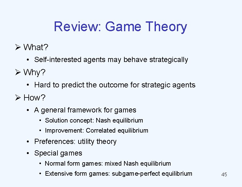
Review: Game Theory Ø What? • Self-interested agents may behave strategically Ø Why? • Hard to predict the outcome for strategic agents Ø How? • A general framework for games • Solution concept: Nash equilibrium • Improvement: Correlated equilibrium • Preferences: utility theory • Special games • Normal form games: mixed Nash equilibrium • Extensive form games: subgame-perfect equilibrium 45