Workshop on Demographic Analysis and Evaluation Mortality Introduction

Workshop on Demographic Analysis and Evaluation

Mortality: Introduction, Measurements, Life Tables

Mortality: Introduction Why do we want to know about mortality? Mortality levels inform us of the health of the population as well as related trends. Mortality age patterns tell us about where targeted investments in health may be especially needed (e. g. , children, elderly, etc. ). Mortality is one of the key components in the balancing equations needed for cohort-component population projections. 3

Mortality: Introduction One of the first steps in making plans for reducing mortality is to know not only the overall level but also the age structure of mortality and, if possible, the main causes of death. Mortality is the second of four components required for population projection (the others being population, fertility, and migration) with the cohort-component method. 4

Mortality In the discussion of mortality in this workshop, we will see that: Mortality estimation may use data from a variety of measurement systems, including vital registration, sample surveys, and census, and may involve a number of procedures. The methods for measuring mortality depend not only on the quality but also on the detail of the information available. If data are reliable, mortality can be estimated directly. If not, then specific techniques are required to estimate mortality indirectly. 5

Mortality: Introduction We will also discuss Life table construction Tools for evaluating the quality of, and for adjusting, deaths data Methods of indirect estimation Derivation and use of a composite mortality series But we begin with measures of mortality and mortality measurement … 6

Mortality: Introduction This discussion follows Chapter 3 of the Census Bureau’s Population Analysis with Microcomputers, which provides more details about the importance of mortality data, techniques for estimating mortality levels and patterns, and methods for adjusting mortality data. 7

Direct Estimation When accurate and reliable information on deaths and population is available from censuses (or vital registration systems), or from questions asked about deaths in a household survey, direct calculations of mortality can be made based on these data. The crude death rate is the most common and the easiest to calculate, but often more complicated measures are needed because they provide additional information. Infant mortality and under-5 mortality are important indicators of a country's development. 8

Direct Estimation Age-specific death rates for other ages are also important in deciding which ages to target for particular programs. Life expectancy at birth (e(0)) is a useful summary measure because it takes into account the mortality situation at each age yet expresses the result in a single figure. 9

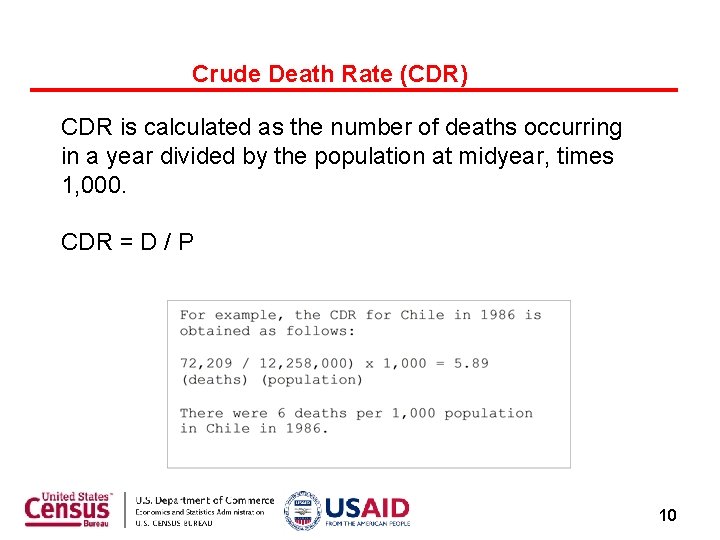
Crude Death Rate (CDR) CDR is calculated as the number of deaths occurring in a year divided by the population at midyear, times 1, 000. CDR = D / P 10

Alternative Measures Because mortality varies with age, a comparison between countries based only on the crude death rate may be misleading. Two populations may have different crude death rates even if mortality at each age is the same in each of them. In another case, one population may actually have lower mortality at each age, and still have a higher crude death rate. An age-standardized crude death rate avoids this problem. 11

Alternative Measures Infant mortality rate, under-5 mortality rate, agespecific mortality rates, and life expectancy at birth also avoid the CDR's problem of confounding age and mortality. 12

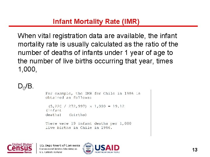
Infant Mortality Rate (IMR) When vital registration data are available, the infant mortality rate is usually calculated as the ratio of the number of deaths of infants under 1 year of age to the number of live births occurring that year, times 1, 000, D 0/B. 13

Infant Mortality Rate (IMR) A more refined rate would take into account a process for relating infant deaths to their actual birth cohort because in reality some of the deaths occurring each year correspond to infants born during the previous year, just as some infants born in the current year will die the following year before reaching their first birthday. The simple calendar-year ratio may provide a good approximation of the IMR; an average of data for three consecutive years may provide a better approximation. 14

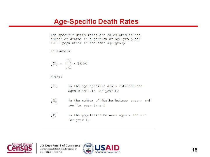
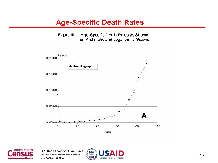
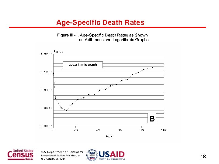
Age-Specific Death Rates While mortality is very high at the early moments of life, it declines rapidly thereafter, reaching its lowest levels between 10 and 15 years of age. At higher ages, the older the age, the higher the mortality generally. Age-specific central death rates are calculated as the number of deaths in a particular age group per 1, 000 population in the same age group: Dx/Px 15

Age-Specific Death Rates 16

Age-Specific Death Rates 17

Age-Specific Death Rates 18

Summarizing the Mortality Level in a Population One of the most useful summary measures of the overall level of mortality of a population is the life expectancy at birth. It is a more accurate reflection of mortality than the crude death rate because it is independent of the population's age structure, and it is not influenced by extraneous factors such as the selection of a standard population. 19

Life Table Construction Calculation of the life expectancy at birth begins with a set of age-specific death rates, from which probabilities of surviving from one age to the next can be estimated. These survival probabilities are applied to an assumed cohort of births that occurred in the same year, following the survivors as they reach successive ages until all have eventually died. 20

Life Table Construction x - 0 1 5 10 15 20 25 30 35 40 45 50 55 60 65 70 75 n n. Mx - - 1 4 5 5 5 5 nax - 0. 1072 0. 0034 0. 0010 0. 0007 0. 0017 0. 0030 0. 0036 0. 0054 0. 0146 0. 0128 0. 0269 0. 0170 0. 0433 0. 0371 0. 0785 0. 0931 nqx - 0. 33 1. 56 2. 50 2. 50 lx - ndx - n. Lx - 0. 100000 10000 93300 0. 0135 90000 1219 357023 0. 0049 88781 438 442809 0. 0037 88343 324 440903 0. 0084 88019 741 438242 0. 0147 87278 1283 433182 0. 0181 85995 1553 426092 0. 0268 84442 2266 416545 0. 0266 82176 2187 405411 0. 0705 79989 5635 385856 0. 0619 74354 4601 360265 0. 1262 69752 8802 326756 0. 0817 60950 4978 292305 0. 1954 55972 10935 252521 0. 1699 45036 7651 206056 0. 3281 37386 12266 156264 0. 3775 25120 9483 101893 5 Px - Tx - 0. 901 0. 983 0. 996 0. 994 0. 988 0. 984 0. 978 0. 973 0. 952 0. 934 0. 907 0. 895 0. 864 0. 816 0. 758 0. 652 0. 569 ex - 5630649 5537349 5180326 4737517 4296614 3858372 3425190 2999097 2582553 2177141 1791286 1431020 1104264 811959 559439 353383 197119 56. 3 61. 5 58. 3 53. 6 48. 8 44. 2 39. 8 35. 5 31. 4 27. 2 24. 1 20. 5 18. 1 14. 5 12. 4 9. 5 7. 8 21

Life Table Construction As a result of this procedure, a count can be obtained of the total number of years that the birth cohort as a whole would live under the observed mortality conditions. The ratio of all years lived by the total number of people in the cohort to the original number of births represents the average number of years to be lived by persons born in the same year under the particular mortality conditions of that year. This ratio is the life expectancy at birth. 22

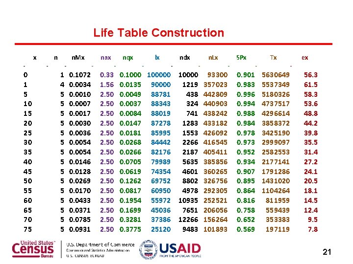
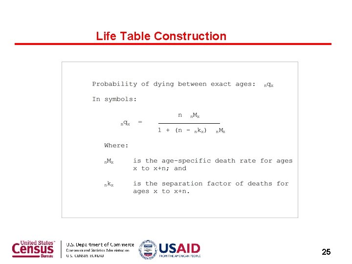
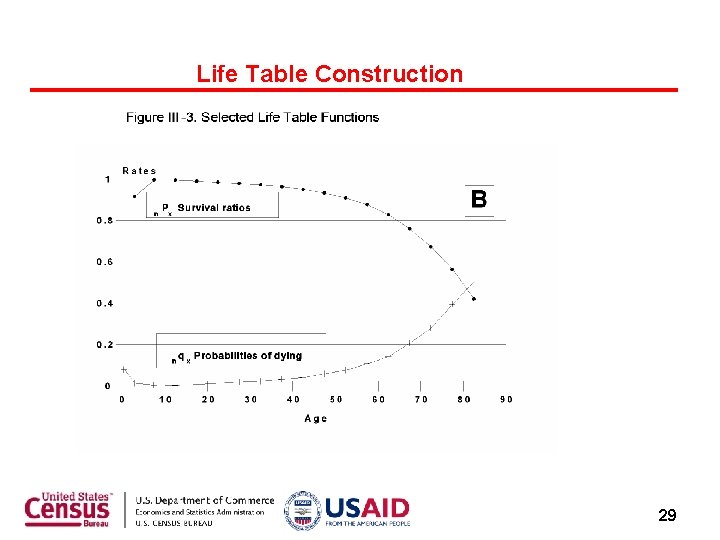
Life Table Construction The construction of a life table consists of calculating various interdependent "functions, " using as a base the available age-specific death rates. The first function calculated in the life table is the probability of dying between two exact ages, for example, the probability that a person of exact age 30 will die before reaching his or her 35 th birthday. This function is symbolized as nqx, where x represents exact age x and n is the age interval. 23

Life Table Construction The probability of dying is obtained by using age-specific death rates and "separation factors" of death. The separation factors represent the average number of years lived during any age interval by persons who die between the defined limits of the age interval. For example, persons who die at age 23 (between exact ages 23 and 24) would live about half that year, on average (since deaths are fairly evenly distributed throughout the year); thus the separation factor in this case would be close to 0. 5. Similarly, when data are presented in 5 -year age groups, separation factors for most age ranges will be close to 2. 5. 24

Life Table Construction 25

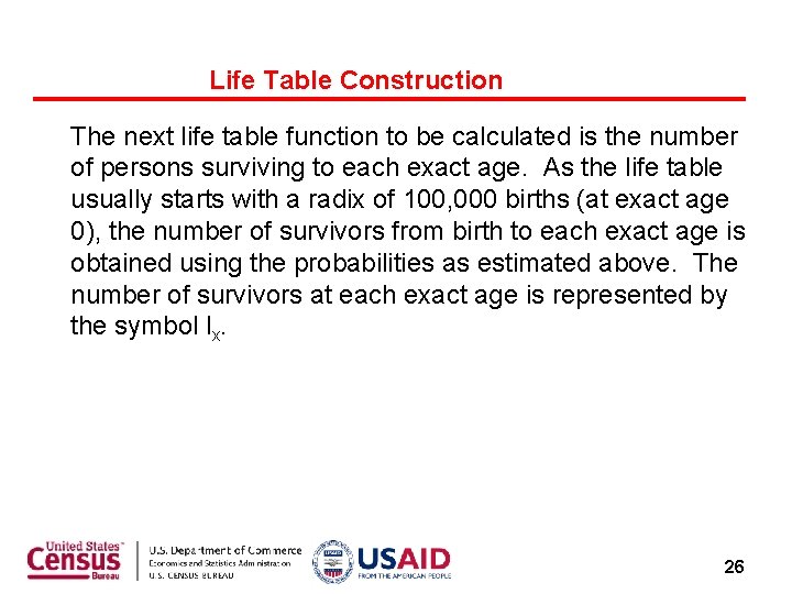
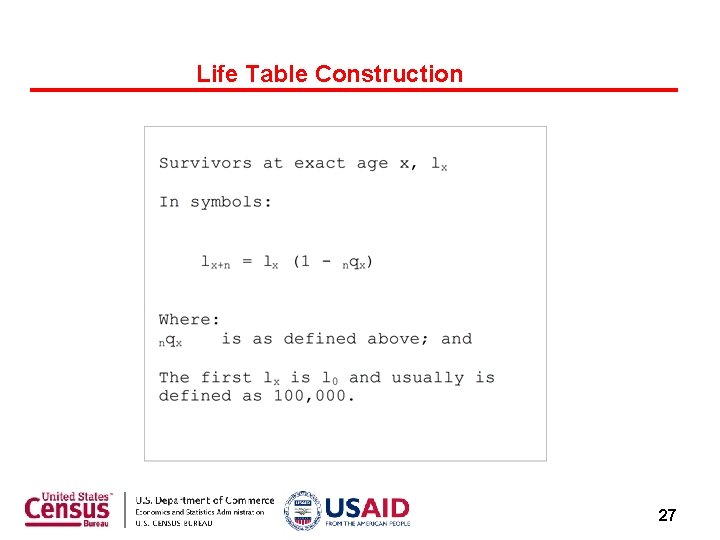
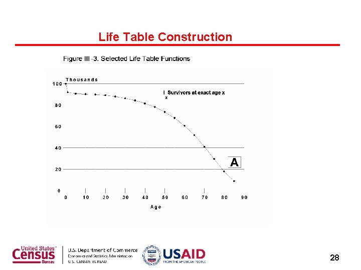
Life Table Construction The next life table function to be calculated is the number of persons surviving to each exact age. As the life table usually starts with a radix of 100, 000 births (at exact age 0), the number of survivors from birth to each exact age is obtained using the probabilities as estimated above. The number of survivors at each exact age is represented by the symbol lx. 26

Life Table Construction 27

Life Table Construction 28

Life Table Construction 29

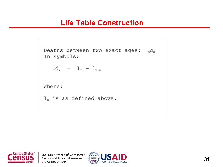
Life Table Construction Since lx represents the number of persons alive at each exact age x, the difference between two consecutive values (for example, lx and lx+n) represents the number of deaths between the corresponding ages (x and x+n, in this case). This number of deaths between two exact ages is symbolized by ndx in the life table. 30

Life Table Construction 31

Life Table Construction Actual populations are usually enumerated in a census or survey as the number of persons alive between two ages, for example, the population at age 23 (persons between their 23 rd and 24 th birthdays) or the population in the age group 15 to 19 years (persons who have reached their 15 th birthday but not yet their 20 th). A life table includes an analogous population, represented by the n. Lx function, referred to as the "life table population" between exact ages x and x+n, or the number of survivors between exact age x and x+n. 32

Life Table Construction The life table population may be interpreted in three different ways: 1. The life table population may be interpreted as a "stationary" population. This means that every year there are 100, 000 births and the same number of deaths, mortality and fertility remain constant, and the number of people in each age group (n. Lx) does not change. 33

Life Table Construction 2. Persons in each particular age group, say 30 to 35 years (5 L 30) may be interpreted as the survivors of 500, 000 births that occurred during a 5 -year period (100, 000 each year) 30 to 35 years ago. 34

Life Table Construction 3. Finally, the total life table age distribution may be interpreted as the survivorship pattern of a single cohort of 100, 000 births as it passes through all ages. In this case, the value of n. Lx in any particular age group represents the number of years that the single cohort of 100, 000 would live between two specific ages, x to x+n. For example, the 5 L 30 value refers to the total number of "person‑years" that 100, 000 births would live between exact ages 30 and 35. 35

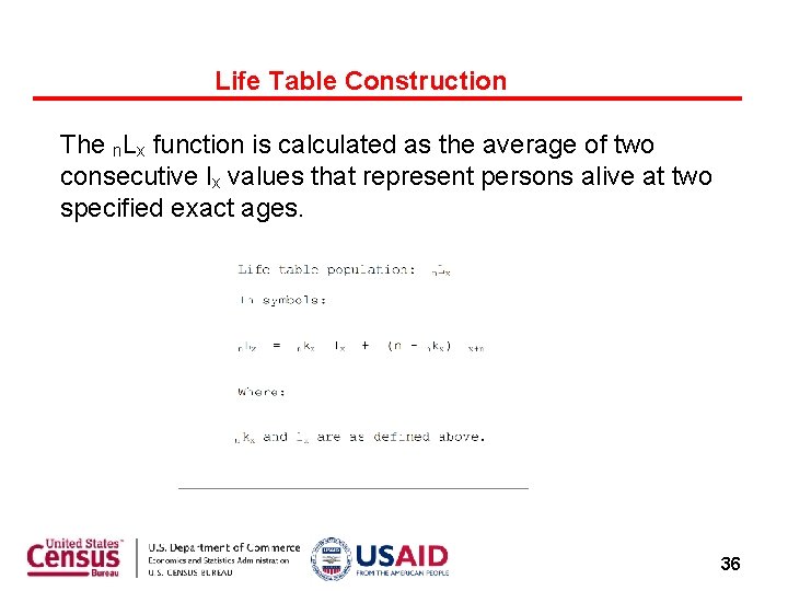
Life Table Construction The n. Lx function is calculated as the average of two consecutive lx values that represent persons alive at two specified exact ages. 36

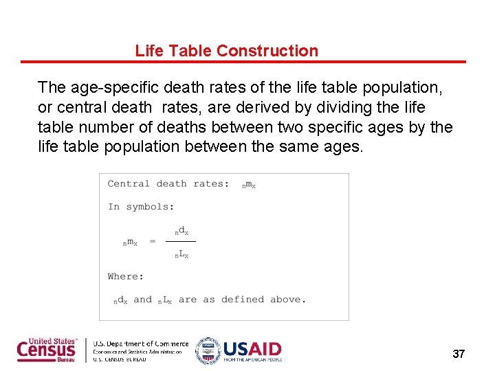
Life Table Construction The age-specific death rates of the life table population, or central death rates, are derived by dividing the life table number of deaths between two specific ages by the life table population between the same ages. 37

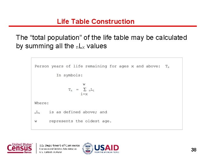
Life Table Construction The “total population” of the life table may be calculated by summing all the n. Lx values 38

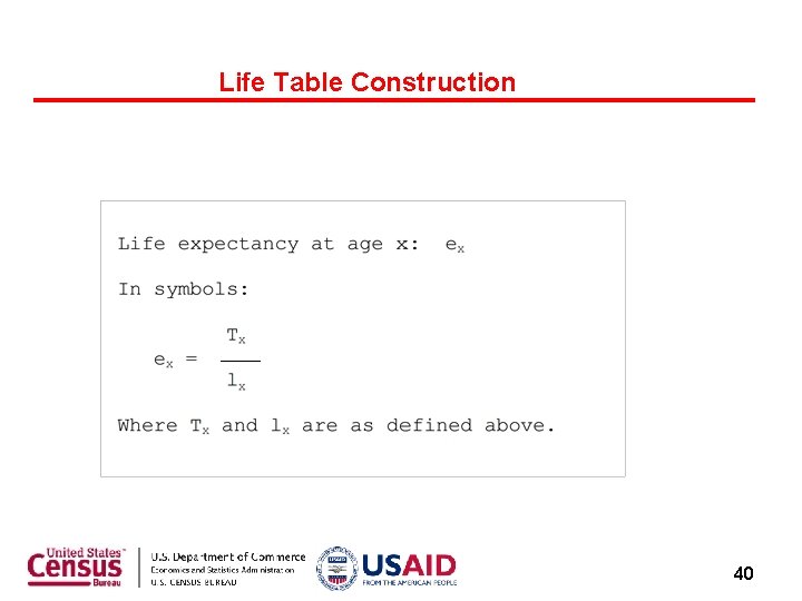
Life Table Construction In the case of an abridged life table, the n. Lx value for the oldest age group (Lw) refers to an open-ended age (85 years and over, for example) and requires selection of a special estimating procedure. Meanwhile, the ratio of the number of person-years that the life table population will live from age x up to the point when all have died, to the number of persons alive at exact age x, represents the average number of years remaining to be lived by those who are alive at each age x. This is the life expectancy at any given age, symbolized by ex. 39

Life Table Construction 40

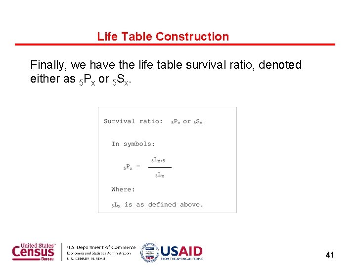
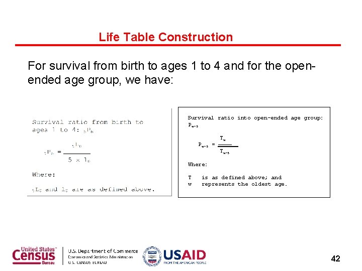
Life Table Construction Finally, we have the life table survival ratio, denoted either as 5 Px or 5 Sx. 41

Life Table Construction For survival from birth to ages 1 to 4 and for the openended age group, we have: Survival ratio into open-ended age group: Pw-5 Tw Pw-5 = Tw-5 Where: T is as defined above; and w represents the oldest age. 42