What is simulation conceive simulation as a special

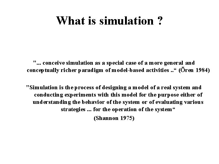
What is simulation ? ". . . conceive simulation as a special case of a more general and conceptually richer paradigm of model-based activities. . “ (Ören 1984) "Simulation is the process of designing a model of a real system and conducting experiments with this model for the purpose either of understanding the behavior of the system or of evaluating various strategies. . . for the operation of the system“ (Shannon 1975)

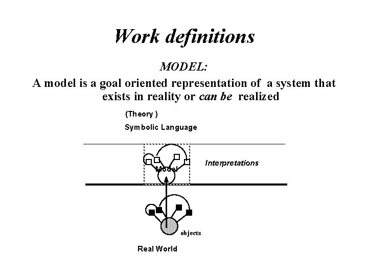
Work definitions MODEL: A model is a goal oriented representation of a system that exists in reality or can be realized (Theory ) Symbolic Language Interpretations Model objects Real World

Work definitions Computermodel: A computer model = an algorithm = of a system that can be realized in the real world Simulation: Simulation is stepping through a computer model with the purpose to describe the behavior of a real system

Paradigms Programs of Research "A scientific view on the world guided by a methodology. . disciplinary matrix. . . symbolic generalization. . shared commitment in a particular model" (Kuhn 1970, 1977) "The history of science has been and should be a history of completing research programs (or if you wish paradigm's ), but it has not been and must become a succession of periods of normal science: the sooner competition starts, the better for progress. Theoretical pluralism is better then theoretical monism" (Lakatos 1970) A successful research program is one that generates a series of theories (a problem shift) which consistently is theoretically progressive and intermittently is empirically progressive. Mature science consists of research programs, whereas immature science consist of a "mere patched up pattern of trial and error" (Lakatos 1970)

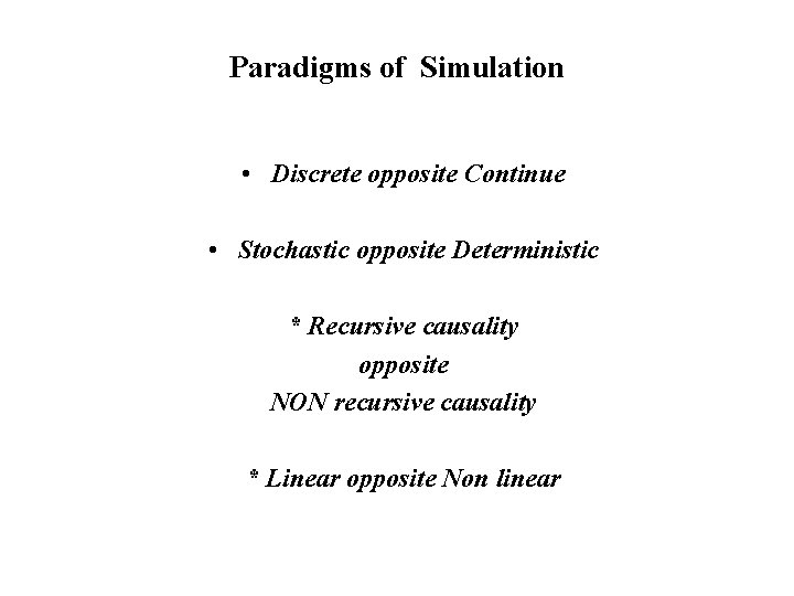
Paradigms of Simulation • Discrete opposite Continue • Stochastic opposite Deterministic * Recursive causality opposite NON recursive causality * Linear opposite Non linear

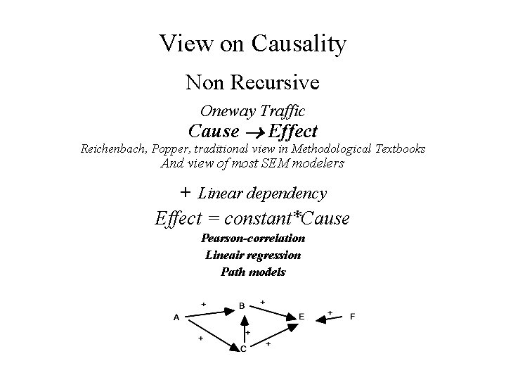
View on Causality Non Recursive Oneway Traffic Cause Effect Reichenbach, Popper, traditional view in Methodological Textbooks And view of most SEM modelers + Linear dependency Effect = constant*Cause Pearson-correlation Lineair regression Path models

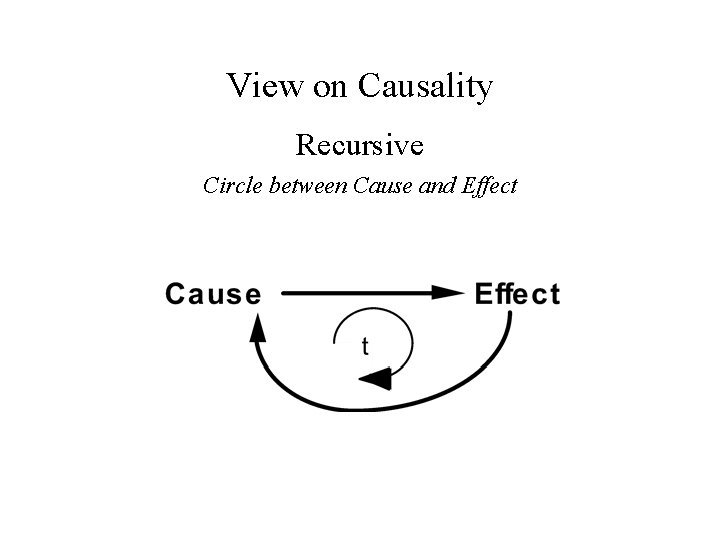
View on Causality Recursive Circle between Cause and Effect

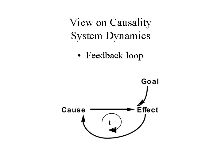
View on Causality System Dynamics • Feedback loop

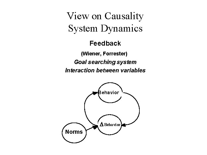
View on Causality System Dynamics Feedback (Wiener, Forrester) Goal searching system Interaction between variables Behavior Norms

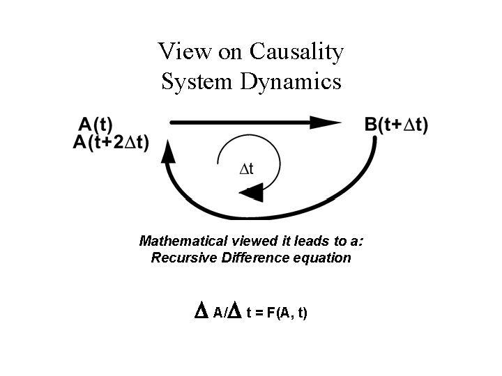
View on Causality System Dynamics Mathematical viewed it leads to a: Recursive Difference equation A/ t = F(A, t)

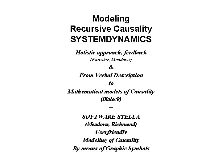
Modeling Recursive Causality SYSTEMDYNAMICS Holistic approach, feedback (Forester, Meadows) & From Verbal Description to Mathematical models of Causality (Blalock) + SOFTWARE STELLA (Meadows, Richmond) Userfriendly Modeling of Causality By means of Graphic Symbols

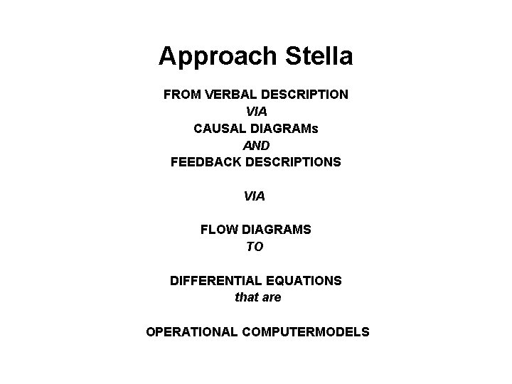
Approach Stella FROM VERBAL DESCRIPTION VIA CAUSAL DIAGRAMs AND FEEDBACK DESCRIPTIONS VIA FLOW DIAGRAMS TO DIFFERENTIAL EQUATIONS that are OPERATIONAL COMPUTERMODELS

STELLA A Demonstration

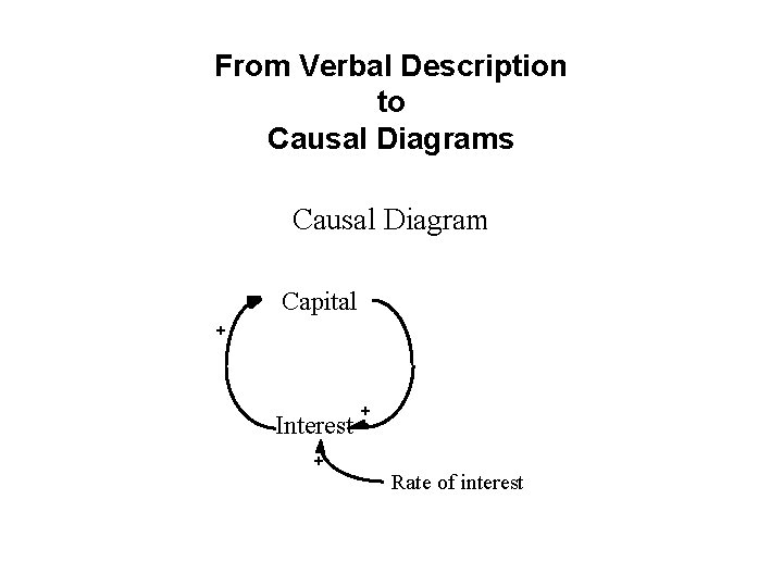
From Verbal Description to Causal Diagrams An Example Verbal Description: Money put on the bank produces after some time interest, that result in more capital on the bank, producing after another period of time -supposing a fixed rate of interest- more interest, and as a consequence more capital, and so on.

From Verbal Description to Causal Diagrams Causal Diagram Capital + + Interest + Rate of interest +

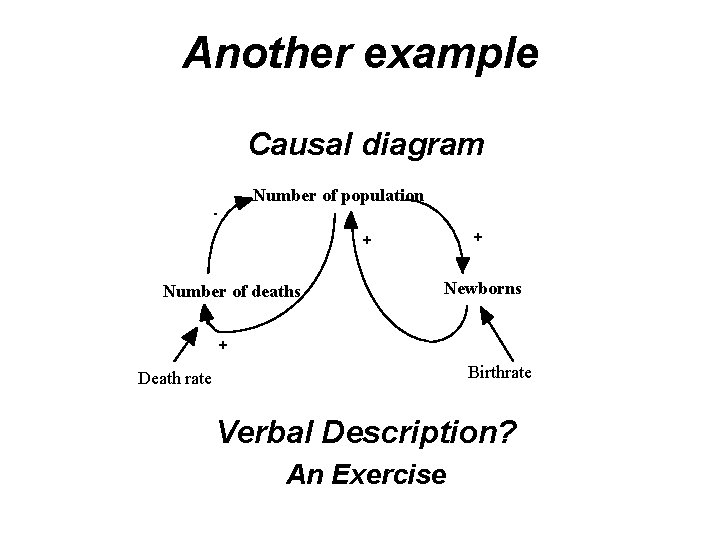
Another example Causal diagram Number of population + + Number of deaths Newborns + Birthrate Death rate Verbal Description? An Exercise

Verbal Description: The number of the newborns and the number of deaths are proportional to the number of the population. The number of newborns is proportional to the birthrate. The number of deaths is proportional to the deathrate. Newborns add up the population. The number of death subtracts from the population (alternative statements are possible)

CAUSAL DESCRIPTIONS Causal diagram

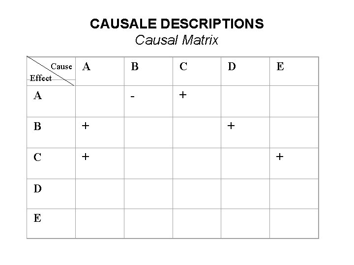
CAUSALE DESCRIPTIONS Causal Matrix A B C D E A - + B + + C + + D E Cause Effect

STELLA • AN EXERCISE – GROWTH OF CAPITAL

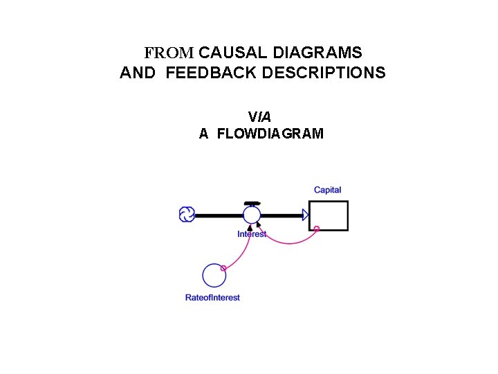
FROM CAUSAL DIAGRAMS AND FEEDBACK DESCRIPTIONS VIA A FLOWDIAGRAM

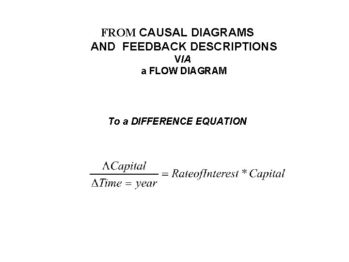
FROM CAUSAL DIAGRAMS AND FEEDBACK DESCRIPTIONS VIA a FLOW DIAGRAM To a DIFFERENCE EQUATION

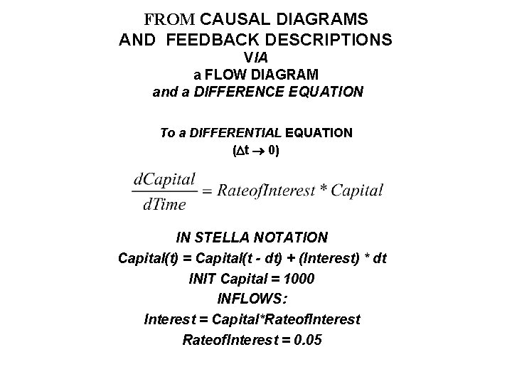
FROM CAUSAL DIAGRAMS AND FEEDBACK DESCRIPTIONS VIA a FLOW DIAGRAM and a DIFFERENCE EQUATION To a DIFFERENTIAL EQUATION ( t 0) IN STELLA NOTATION Capital(t) = Capital(t - dt) + (Interest) * dt INIT Capital = 1000 INFLOWS: Interest = Capital*Rateof. Interest = 0. 05

Differential Equations Linear Differential Equations – An Exercise – Growth of a Population

Differential Equations Non Linear Differential Equations – An Exercise – Limited Growth of a Population

Differential Equations Non Linear Differential Equations – An Exercise Spread of a disease

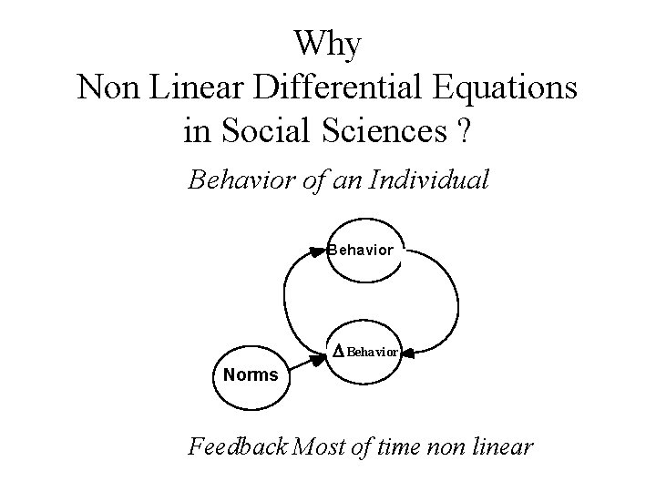
Why Non Linear Differential Equations in Social Sciences ? Behavior of an Individual Behavior Norms Feedback Most of time non linear

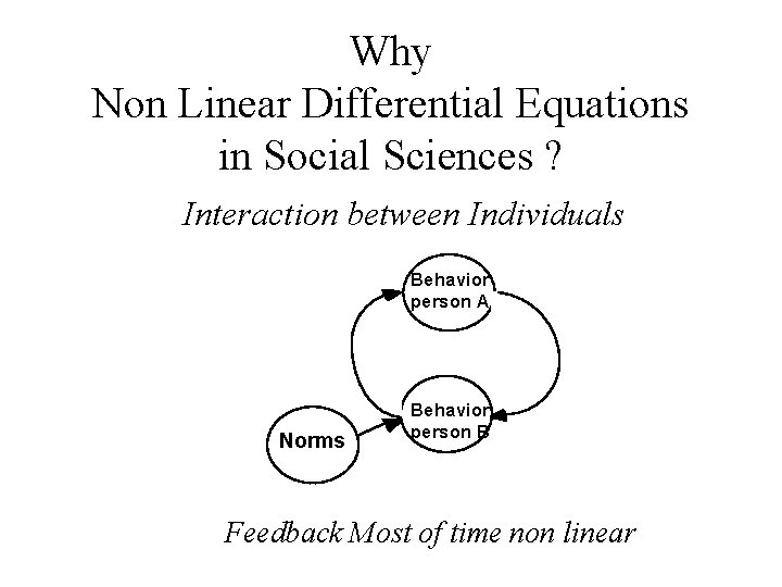
Why Non Linear Differential Equations in Social Sciences ? Interaction between Individuals Behavior person A Norms Behavior person B Feedback Most of time non linear

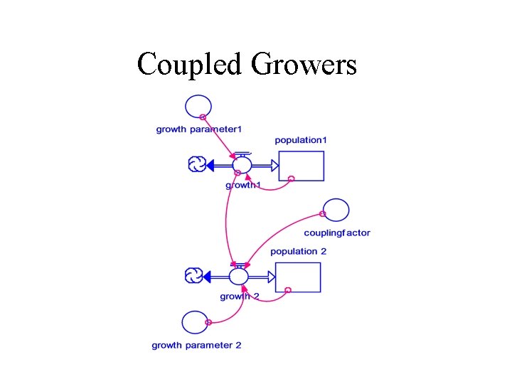
Differential Equations Non Linear Differential Equations – An Exercise Coupled Limited Growth

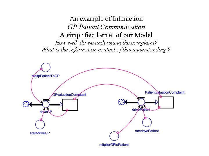
An example of Interaction GP Patient Communication A simplified kernel of our Model How well do we understand the complaint? What is the information content of this understanding ?

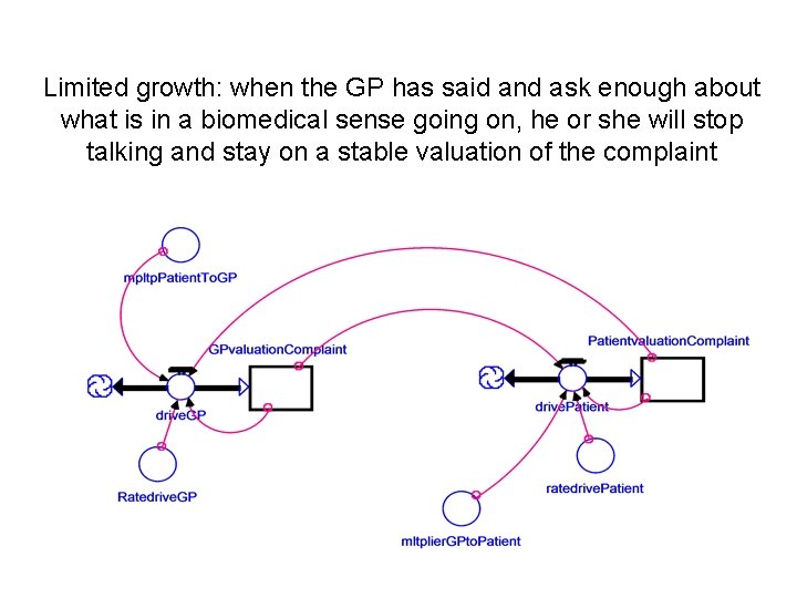
Limited growth: when the GP has said and ask enough about what is in a biomedical sense going on, he or she will stop talking and stay on a stable valuation of the complaint

When patients need to understand Limited growth: when the Patient has asked and said enough about what is in a biomedical sense going on, he or she will stop talking and stay on a stable valuation of the complaint But those two interact!

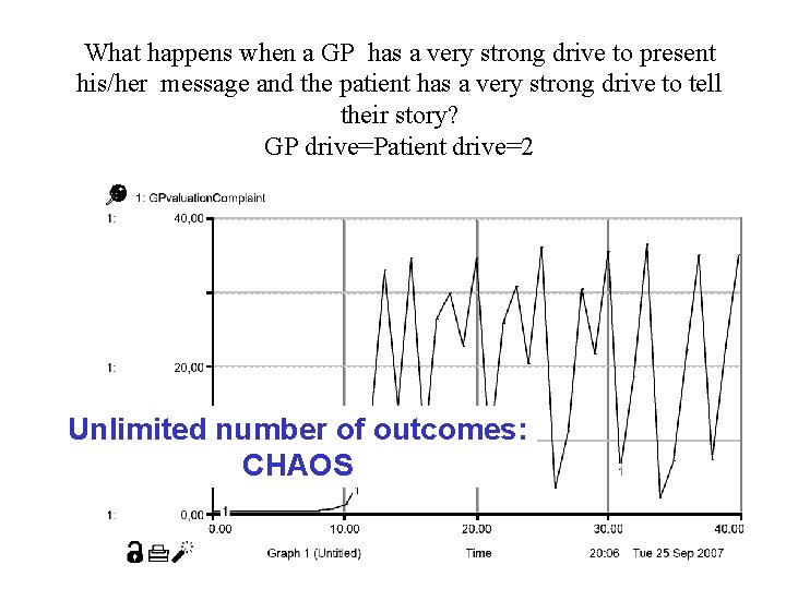
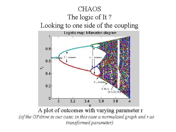
What happens when a GP has a very strong drive to present his/her message and the patient has a very strong drive to tell their story? GP drive=Patient drive=2 Unlimited number of outcomes: CHAOS

CHAOS The logic of It ? Looking to one side of the coupling To A plot of outcomes with varying parameter r (of the GPdrive in our case; in this case a normalized graph and r as transformed parameter)

Coupled Growers

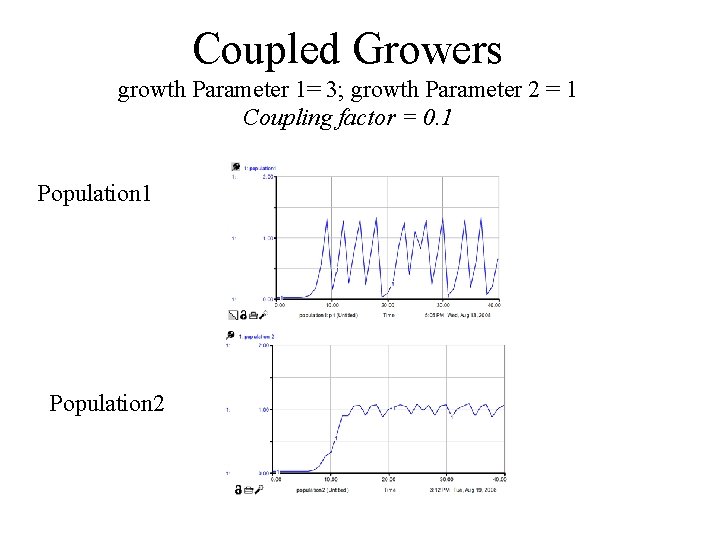
Coupled Growers growth Parameter 1= 3; growth Parameter 2 = 1 Coupling factor = 0. 1 Population 2

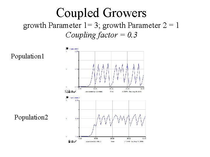
Coupled Growers growth Parameter 1= 3; growth Parameter 2 = 1 Coupling factor = 0. 3 Population 1 Population 2

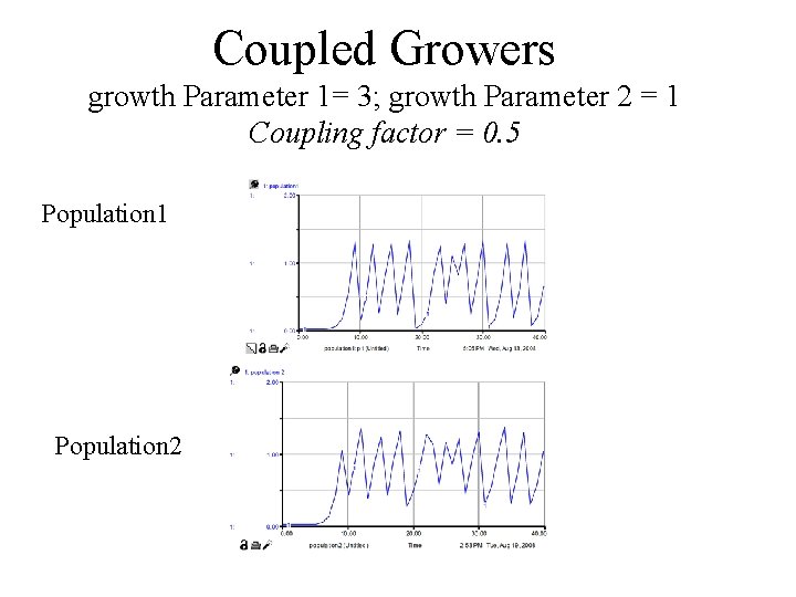
Coupled Growers growth Parameter 1= 3; growth Parameter 2 = 1 Coupling factor = 0. 5 Population 1 Population 2

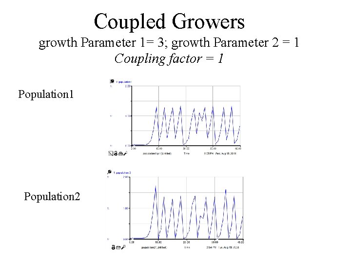
Coupled Growers growth Parameter 1= 3; growth Parameter 2 = 1 Coupling factor = 1 Population 2

Coupled Growers Effects Plot of changing coupling factor And output population 1 and 2 ? ! For this STELLA is not suited USE MATLAB

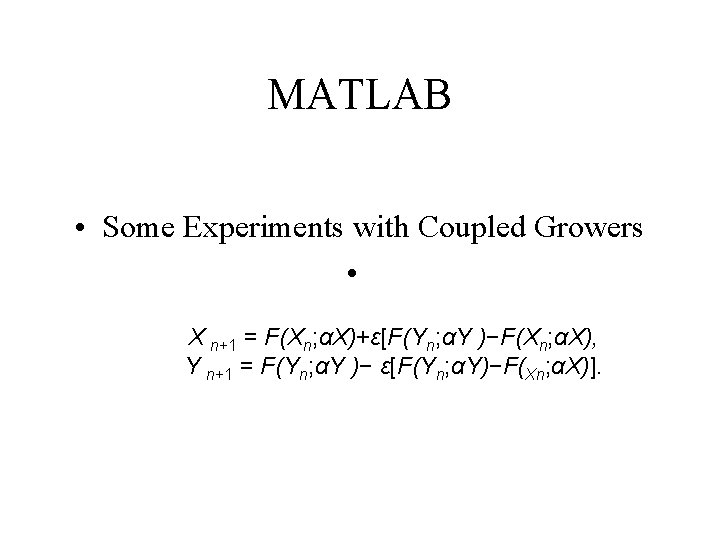
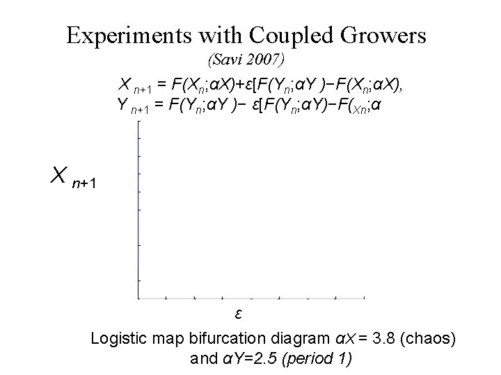
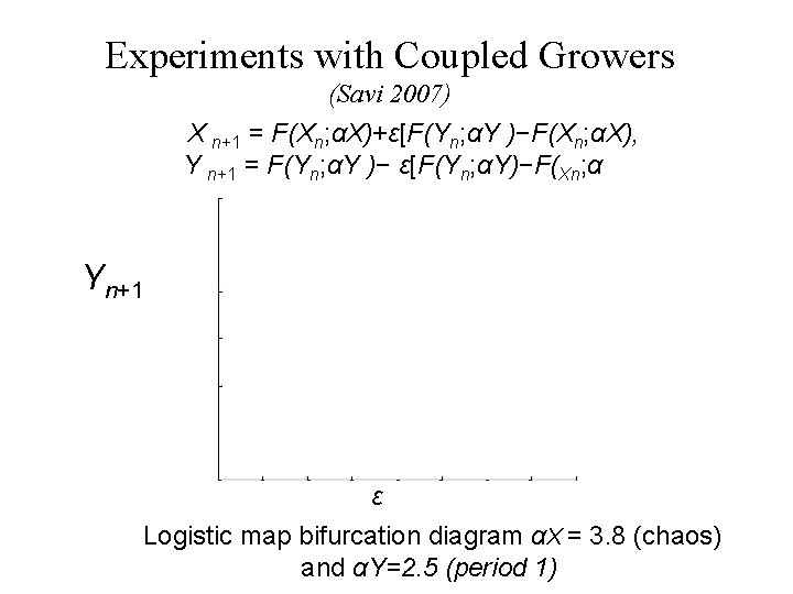
MATLAB • Some Experiments with Coupled Growers • X n+1 = F(Xn; αX)+ε[F(Yn; αY )−F(Xn; αX), Y n+1 = F(Yn; αY )− ε[F(Yn; αY)−F(Xn; αX)].

Experiments with Coupled Growers (Savi 2007) X n+1 = F(Xn; αX)+ε[F(Yn; αY )−F(Xn; αX), Y n+1 = F(Yn; αY )− ε[F(Yn; αY)−F(Xn; αX)]. X n+1 ε Logistic map bifurcation diagram αX = 3. 8 (chaos) and αY=2. 5 (period 1)

Experiments with Coupled Growers (Savi 2007) X n+1 = F(Xn; αX)+ε[F(Yn; αY )−F(Xn; αX), Y n+1 = F(Yn; αY )− ε[F(Yn; αY)−F(Xn; αX)]. Yn+1 ε Logistic map bifurcation diagram αX = 3. 8 (chaos) and αY=2. 5 (period 1)

Some Literature • • • Barlas, Y. 1989. “Multiple Tests for Validation of System Dynamics Type of Simulation Models. ” European Journal of Operational Research 42(1): 59 -87. Dijkum C. van (2001). A Methodology for Conducting Interdisciplinary Social Research. European Journal of Operational Research, Vol. 128, Iss. 2, 290 -299. Dijkum C. van, Landsheer H. (2000). Experimenting with a Non-linear Dynamic Model of Juvenile Criminal Behavior. Simulation & Gaming, Vol. 31, No. 4, 479 -490. Dijkum C. , Mens-Verhulst J. van, Kuijk E. van, Lam N. (2002), System Dynamic Experiments with Non-linearity and a Rate of Learning, Journal of Artificial Societies and Social Simulation, Vol. 5, 3. Dijkum, C. van, Verheul W. Bensing J. , Lam N. , Rooi J. de (2008). “Non Linear Models for the Feedback between GP and Patients. ” In Cybernetics and Systems. Trappl R. (ed). Vienna: Austrian Society for Cybernetic Studies. (download: http: //www. nosmo. nl/rc 33/nonlinear. pdf) Forrester, J. W. (1968). Principles of Systems. Cambridge MA: Wright-Allen Press.

Some Literature • • Haefner J. W. (1996). Modeling biological systems. New York: Chapman & Hall. Hanneman, R. A (1988). Computer-assisted theory building: Modeling dynamic social systems. Newbury Park: Sage. Richardson, G. P. and A. L. Pugh III. 1981. Introduction To System Dynamics Modeling With DYNAMO. Portland, OR: Productivity Press. Schroots J. , Dijkum C. van (2004). Autobiographical Memory Bump- A Dynamic Lifespan Model. Dynamical Psychology: An International, Interdisciplinary Journal of Complex Mental Processes. (http: //www. goertzel. org/dynapsyc/dynacon. html)