Unit 2 Demand Revenue Analysis Unit 2 Demand

Unit -2 Demand & Revenue Analysis

Ø Unit 2 : Demand Analysis • Concept of Demand • Elasticity of Demand their types. • Revenue Concepts - Total Revenue, Marginal Revenue, Average Revenue and their relationship.

INTRODUCTION Ø It is essential for the business managers to have a clear understanding of the following aspects of the demand for their products : • What are the sources of demand? • What are the determinants of demand? • How do the buyers decide the quantity of a product to be purchased? • How do the buyers respond to the change in a product prices, their income and prices of the related goods? • How can the total of market demand for a product be assessed and forecast? Ø These questions are answered by the Theory of Demand.

MEANING OF DEMAND Ø The term ‘demand’ means a ‘desire’ for a commodity backed by ability and willingness to pay for it. Ø A want with three attributes - desire to buy, willingness to pay and ability to pay - becomes effective demand. Only an effective demand figures in economic analysis and business decisions. Ø The term ‘demand’ for a commodity (i. e. , quantity demanded) has always a reference to ‘a price’, ‘a period of time’ and ‘a place’.

DETERMINANTS OF MARKET DEMAND Ø Price of the goods : higher the price less will be demanded and vise-versa Ø Income: A rise in a person’s income will lead to an increase in demand. Ø Consumer Preferences: Favorable change leads to an increase in demand, unfavorable change lead to a decrease. Ø Number of Buyers: the more buyers lead to an increase in demand; fewer buyers lead to decrease. Ø Price of related goods: • a. Substitute goods (those goods that can be used to replace each other): price of substitute and demand for the other good are directly related. • Example: If the price of coffee rises, the demand for tea should increase. • b. Complement goods (those goods that can be used together): price of complement and demand for the other good are inversely related. • Example: if the price of petrol rises, the demand for cars will decrease. Ø Expectation of future: • a. Future price: consumers’ current demand will increase if they expect higher future prices; their demand will decrease if they expect lower future prices. • b. Future income: consumers’ current demand will increase if they expect higher future income; their demand will decrease if they expect lower future income.

THE LAW OF DEMAND Ø The law of demand states that the demand for a commodity increases when its price decreases and it falls when its price rises, other things remaining constant. (ceteris paribus) Ø The law reveals, there is an inverse relationship between the price and quantity demanded. Ø The law holds under the condition that “other things remain constant”. “Other things” include other determinants of demand, viz. , consumers’ income, price of the substitutes and complements, taste and preferences of the consumer, etc.

Demand Schedule • The law of demand can be presented through a demand schedule. • Demand Schedule is a series of prices placed in descending (or ascending) order and the corresponding quantities which consumers would like to buy per unit of time. Price per cup of tea (Rs. ) consumer No. of cups of Tea demand by a per day combination Points representing price -quantity 7 1 i 6 2 j 5 3 K 4 4 l 3 5 m 2 6 n 1 7 o

Demand Curve • The law of demand can also be presented through a demand curve. A demand curve is a locus of points showing various alternative price quantity combinations. Demand curve shows the quantities of a commodity which a consumer would buy at different prices.

Factors behind the Law of Demand Ø Substitution Effect : • When price of a commodity falls, prices of all other related goods (particularly of substitutes) remaining constant, the goods of latter category become relatively costlier. Or, in other words, the commodity whose price has fallen becomes relatively cheaper. The increase in demand on account of this factor is known a substitution effect. Ø Income Effect : • As a result of fall in the price of a commodity, the real income of the consumer increases. Consequently, his purchasing power increases since he is required to pay less for the same quantity. The increase in real income encourages the consumer to demand more of goods and services. The increase in demand on account of increase in real income is known as income effect.

Exceptions to the Law of Demand • Expectations regarding further prices: When consumers expect a continuous increase in the price of a durable commodity, they buy more of it despite increase in its price with a view to avoiding the pinch of a much higher price in future. • Veblen Goods: The law does not apply to the commodities which are used as a status symbol’ of enhancing social prestige or for displaying wealth and riches, e. g. , gold, ’ precious stones, rare paintings, antiques, etc. • Inferior goods : are those goods whose demand decreases as income of the consumer increase. Therefore if the price of inferior goods decrease it doesn’t increase the quantity mainly because consumers’ real income increases and they become relatively richer: Consequently, they substitute the superior goods for the inferior ones. • Giffen goods : Sir Robert Giffen who observed that when the price of bread increased, the low paid British workers in the early 19 th century purchased more bread and not less of it. The reason given for this is that these British workers consume a diet of mainly bread and therefore , they could not afford to purchase as much other goods before.

Elasticity of demand Ø Elasticity measures the degree of responsiveness of demand to the changes in its determinants. Ø In this section, we will discuss various methods of measuring elasticity of demand. The concepts of demand elasticity used in business decisions are: (i) Price-elasticity; (ii) Cross-elasticity; (iii) Income-elasticity;

PRICE ELASTICITY OF DEMAND Ø Price elasticity of demand is generally defined as the responsiveness or sensitiveness of demand for a commodity to the changes in its price. More precisely, elasticity of demand is the percentage changes in demand as a result of one per cent in the price of the commodity. Ø A formal definition of price-elasticity of demand (ep) is given as Percentage change in quantity demanded ————————— Percentage change in price Ø ep = Ø A general formula for calculating coefficient of price-elasticity, derived from this definition of elasticity, is given as follows Q 2 -Q 1 ∆ Q 1 EP = --------Q 1 Q 2 + Q 1 ------ or ----- ( Modified version) P 2 – P 1 ∆ P 1 Ø ------------------ P 2 + P 1 where Q 1 = original quantity demanded, P 1 = original price, Q 2 = change in quantity demanded, and P 2 = change in price.

Ø It is important to note here that, a minus sign (-) is generally inserted in the formula before the fraction with a view to making elasticity coefficient a nonnegative value.

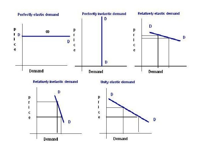
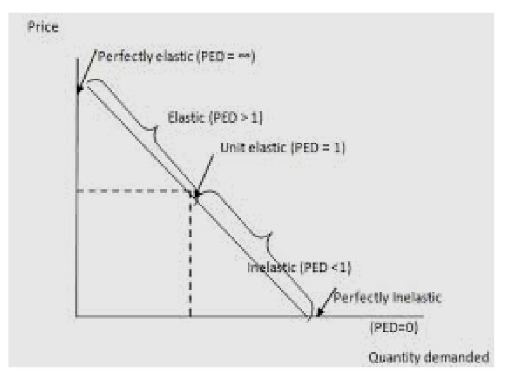
Types of Price Elasticity Types Numerical Expression Description Shape of the curve Perfectly Elastic ∞ Infinite Horizontal Perfectly Inelastic 0 zero Vertical Unity Elasticity 1 One Rectangular Hyperbola Relatively Elastic ˃1 More than one Flat Relatively Inelastic ˂1 Less than one Steep

Ø Perfectly elastic demand: • The demand is said to be perfectly elastic when a very insignificant change in price leads to an infinite change in quantity demanded. • A very small fall in price causes demand to rise infinitely. Likewise a very insignificant rise in price reduces the demand to zero. This case is theoretical which is never found in real life. Ø Perfectly inelastic demand: • The demand is said to be perfectly inelastic when a change in price produces no change in the quantity demanded of a commodity. • In such a case quantity demanded remains constant regardless of change in price. The amount demanded is totally unresponsive of change in price. The elasticity of demand is said to be zero.

Ø Unitary elastic demand: • The demand is said to be unit when a change in price produces exactly the same percentage change in the quantity demanded of a commodity. • In such a situation the percentage change in both the price and quantity demanded is the same. • For example if the price falls by 25% the quantity demanded rises by the same 25%. It takes the shape of a rectangular hyperbola. Numerically elasticity of demand is said to be equal to 1. (ed = 1). Ø Relatively elastic demand: • The demand is relatively more elastic when a small change in price causes a greater change in quantity demanded. In such a case a proportionate change in price of a commodity causes more than proportionate change in quantity demanded. If price changes by 10% the quantity demanded of the commodity change by more than 10% i. e. 25%. The demand curve in such a situation is relatively flatter.

Ø Relatively inelastic demand: • It is a situation where a greater change in price leads to smaller change in quantity demanded. The demand is said to be relatively inelastic when a proportionate change in price is greater than the proportionate change in quantity demanded. For example If price falls by 20% quantity demanded rises by less than 20% i. e 15%.

Factors Determining Price elasticity of demand Ø Nature of the commodity : The demand for the necessities is generally inelastic and demand for luxuries are elastic. Ø Extent of Use : A commodity having multiple uses has a comparatively elastic demand. For e. g Steel. Ø Range of Substitutes : A commodity having a number of substitute has relatively elastic demand. Ø Income Level : the demand for goods and service are inelastic for rich but elastic for poor. Ø Durability of a commodity : More durable and repairable a commodity is, the higher is its elasticity of demand likely to be. Ø Proportion of income spent on the commodity : where an individual spends only a small portion of his income on the commodity, the price change does not affect his demand for the commodity. For e. g match box, salt, etc.

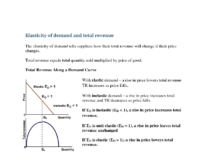
Business Application of price elasticity Ø The effect of a change in price on the total revenue & expenditure on a product. Ø The price volatility in a market following changes in supply – this is important for commodity producers who suffer big price and revenue shifts from one time period to another. Ø The effect of a change in an indirect tax on price and quantity demanded and also whether the business is able to pass on some or all of the tax onto the consumer. Ø Information on the PED can be used by a business as part of a policy of price discrimination. This is where a supplier decides to charge different prices for the same product to different segments of the market e. g. peak and off peak rail travel or prices charged by many of our domestic and international airlines. Ø Usually a business will charge a higher price to consumers whose demand for the product is price inelastic.

Income Elasticity of demand Ø Income Elasticity may be defined as the degree of responsiveness of quantities demanded to a given change in income. The income elasticity of demand can be measured by the following formula ey = Ø or Prop. Change in Quantities demanded -------------------------Prop. Change in Incomes Q 2 -Q 1 -----Q 2 + Q 1 ----------- Y 2 -Y 1 ----------- Y 2 +Y 1 Ø where Q 1 = original quantity demanded, Y 1 = original Income Q 2 = change in quantity demanded, and Y 2 = change in Change In Income Ø Suppose a consumer’s income is Rs. 1, 000 and he purchases ten kilos of sugar. If his income goes up to Rs. 1, 100, he is prepared to buy 12 kilos of sugar. The income elasticity of demand will be. . ?

• Suppose a consumer’s income is Rs. 1, 000 and he purchases ten kilos of sugar. If his income goes up to Rs. 1, 100, he is prepared to buy 12 kilos of sugar. The income elasticity of demand will be. . ? 12 -10 ----------- ey = 12+ 10 2 100 ------- / ----1, 100 -1, 000 22 2, 100 ---------1, 100+ 1, 000 = 1. 99

Types of Income Elasticity Ø Zero Income : Change in Income will have no effect on the quantity demanded. For e. g Salt. Ø Negative Income Elasticity : An increase in income leads to decrease in quantity demanded. For e. g Inferior goods Ø Positive Income Elasticity : An increase in income may lead to an increase in the quantities demanded. For most goods, the income elasticity of demand is positive. Ø Positive Income elasticity can be three Kinds : 1) Unity Elasticity 2) More than Unity Elasticity 3) Less than unity Elasticity

Types of Income Elasticity Value of Co-efficient High Income elasticity Ey= ˃1 Low Income Elasticity Ey = ˂1 Unity Elasticity Ey = 1 Zero Income Elasticity Ey = 0 Negative Income Elasticity Ey = ˂ 0

Types of Income Elasticity Ey=0 Ey=1 Income Quantity Demanded Ey ˃ 1 Income Quantity Demanded Ey<1 Quantity Demanded Ey ˂ 1 Income Quantity Demanded

Cross Elasticity of Demand • Cross Elasticity of demand may be defined as “ The proportionate change in the quantity demanded of a particular commodity in response to change in the price of another related commodity. ” the cross Elasticity of demand can be measured by the following formula : • Qx 2 – Qx 1 ------------ ep= Qx 2+Qx 1 Prop. Change in the quantity purchased of x ----------- = ---------------------------Pz 2 -Pz 1 Prop. Change in the price charged for z -----------Pz 2+Pz 1

• If cross elasticity is positive , the goods are said to be substitutes if negative , the goods are complementary. Unrelated Goods Substitute Price Complements Quantity Demanded

Revenue Analysis Ø In business, revenue or turnover is income that a company receives from its normal business activities, usually from the sale of goods and services to customers. Ø Revenue Concepts : • Total Revenue : Total revenue , means the total sales proceeds. It can be ascertained by multiplying quantities sold by price. TR= Q*P (Q= Quantity, P= Price) • Average Revenue : It means the total receipt from sales divided by the number of units sold. AR = TR/Q ( TR= Total Revenue , Q= Quantity) • Marginal Revenue: Revenue earned by selling additional unit of output is called as marginal revenue. In other words, change in the revenue resulting from a one unit increase in output is marginal revenue. Symbolically, MR = TRn - TR n-1 Where MR = Marginal Revenue TR = Total Revenue n = Unit sold

Relationship between TR, AR, & MR Quantity Demanded Total Revenue 1 9 2 16 3 21 4 24 5 25 6 24 7 21 8 16 9 9 Average Revenue Marginal Revenue

Relationship between TR, AR, & MR Quantity Demanded Total Revenue Average Revenue Marginal Revenue 1 9 9 9 2 16 8 7 3 21 7 5 4 24 6 3 5 25 5 1 6 24 4 -1 7 21 3 -3 8 16 2 -5 9 9 1 -7 1. So long the average revenue is falling, marginal revenue will be less than the average revenue. 2. Marginal revenue falls more steeply than average revenue. 3. Total revenue will be rising so long as marginal revenue is positive. 4. Where marginal revenue is negative, total revenue must be falling 5. Total revenue will be the maximum at a point where marginal revenue is positive and minimum.