The Multistrand Simulator Stochastic Simulation of the Kinetics

The Multistrand Simulator: Stochastic Simulation of the Kinetics of Multiple Interacting DNA Strands Joseph Schaeffer, Caltech (slides by John Reif)

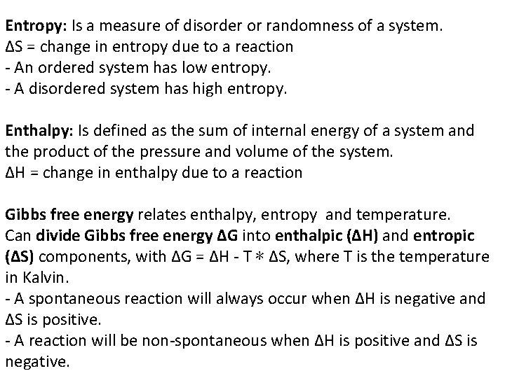
Entropy: Is a measure of disorder or randomness of a system. ∆S = change in entropy due to a reaction - An ordered system has low entropy. - A disordered system has high entropy. Enthalpy: Is defined as the sum of internal energy of a system and the product of the pressure and volume of the system. ∆H = change in enthalpy due to a reaction Gibbs free energy relates enthalpy, entropy and temperature. Can divide Gibbs free energy ∆G into enthalpic (∆H) and entropic (∆S) components, with ∆G = ∆H - T ∗ ∆S, where T is the temperature in Kalvin. - A spontaneous reaction will always occur when ∆H is negative and ∆S is positive. - A reaction will be non-spontaneous when ∆H is positive and ∆S is negative.

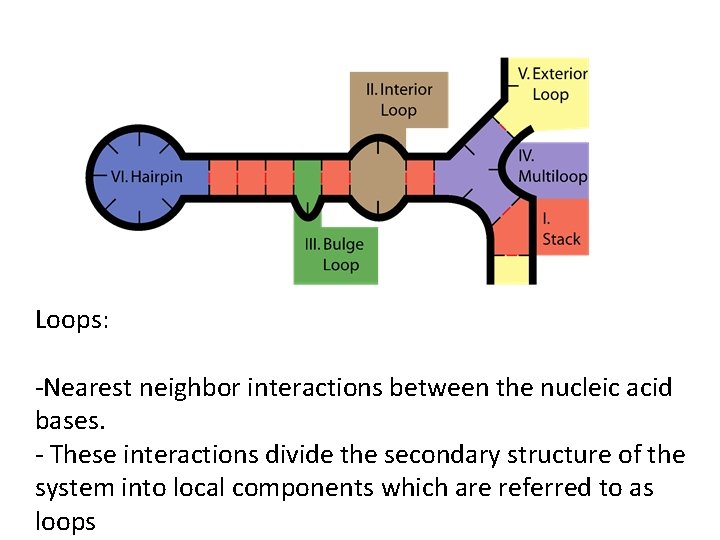
Loops: -Nearest neighbor interactions between the nucleic acid bases. - These interactions divide the secondary structure of the system into local components which are referred to as loops

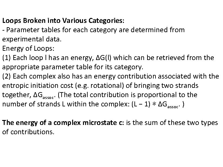
Loops Broken into Various Categories: - Parameter tables for each category are determined from experimental data. Energy of Loops: (1) Each loop l has an energy, ∆G(l) which can be retrieved from the appropriate parameter table for its category. (2) Each complex also has an energy contribution associated with the entropic initiation cost (e. g. rotational) of bringing two strands together, ∆Gassoc. (The total contribution is proportional to the number of strands L within the complex: (L − 1) ∗ ∆Gassoc. ) The energy of a complex microstate c: is the sum of these two types of contributions.

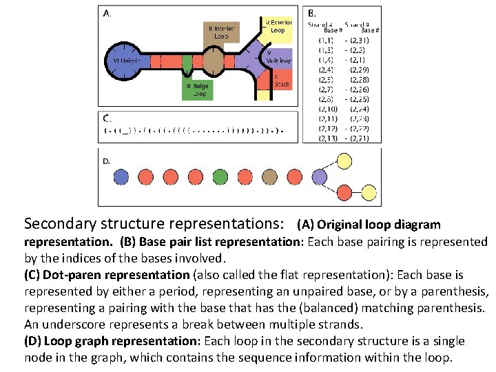
Secondary structure representations: (A) Original loop diagram representation. (B) Base pair list representation: Each base pairing is represented by the indices of the bases involved. (C) Dot-paren representation (also called the flat representation): Each base is represented by either a period, representing an unpaired base, or by a parenthesis, representing a pairing with the base that has the (balanced) matching parenthesis. An underscore represents a break between multiple strands. (D) Loop graph representation: Each loop in the secondary structure is a single node in the graph, which contains the sequence information within the loop.

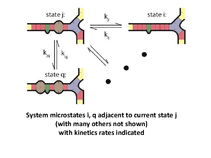
System microstates i, q adjacent to current state j (with many others not shown) with kinetics rates indicated

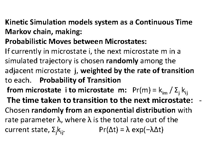
Kinetic Simulation models system as a Continuous Time Markov chain, making: Probabilistic Moves between Microstates: If currently in microstate i, the next microstate m in a simulated trajectory is chosen randomly among the adjacent microstate j, weighted by the rate of transition to each. Probability of Transition from microstate i to microstate m: Pr(m) = kim / Σj kij The time taken to transition to the next microstate: - Chosen randomly from an exponential distribution with rate parameter λ, where λ is the total rate out of the current state, Σjkij. Pr(∆t) = λ exp(−λ∆t)

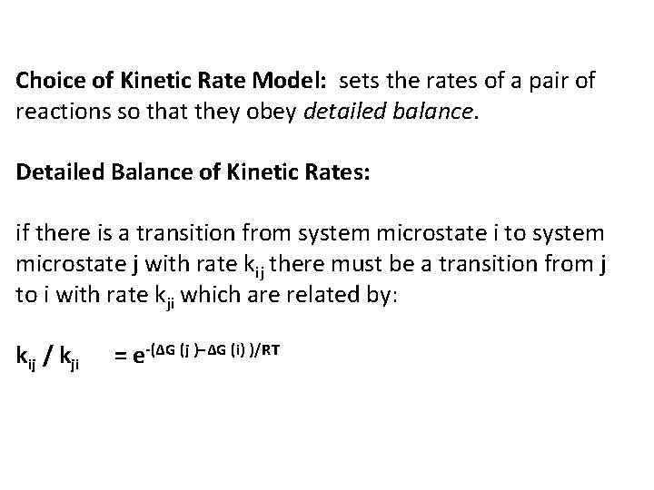
Choice of Kinetic Rate Model: sets the rates of a pair of reactions so that they obey detailed balance. Detailed Balance of Kinetic Rates: if there is a transition from system microstate i to system microstate j with rate kij there must be a transition from j to i with rate kji which are related by: kij / kji = e-(∆G (j )−∆G (i) )/RT

Classify transitions between microstates into two exclusive types: Unimolecular Transitions: Transitions where changes are within a single complex. Bimolecular Transitions: Transitions that change the number of complexes present in the system.

Unimolecular Transitions: transitions between microstates where changes are within a single complex. - Define these transitions in terms of the complex microstate which changed, rather than the full system microstate. - Define a complex microstate d as being adjacent to a complex microstate c if it differs by exactly one base pair. Creation Move: a transition from c to d that adds a base pair a. Deletion Move: transition from c to d that removes a base pair a.

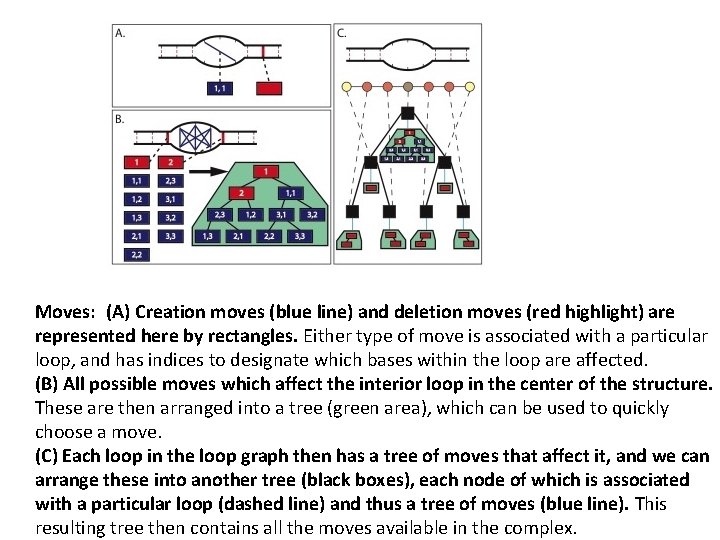
Moves: (A) Creation moves (blue line) and deletion moves (red highlight) are represented here by rectangles. Either type of move is associated with a particular loop, and has indices to designate which bases within the loop are affected. (B) All possible moves which affect the interior loop in the center of the structure. These are then arranged into a tree (green area), which can be used to quickly choose a move. (C) Each loop in the loop graph then has a tree of moves that affect it, and we can arrange these into another tree (black boxes), each node of which is associated with a particular loop (dashed line) and thus a tree of moves (blue line). This resulting tree then contains all the moves available in the complex.

Unimolecular Rate Models: Kawasaki method: both “downhill” (energetically favorable) and uphill transitions scale directly with the steepness of their slopes. (There is no bound on the maximum rate. ) Metropolis method: all downhill moves occur at the same fixed rate, and only the uphill moves scale with the slope. (Maximum rate for any move is bounded, and all downhill moves occur at this rate. ) Entropy/Enthalpy Method: uses the division of free energies into entropic and enthalpic components to assign the transition rates in an intuitive manner: base pair creation moves must overcome the entropic energy barrier to bring the bases into contact, and base pair deletion moves must overcome the enthalpic energy barrier in order to break them apart.

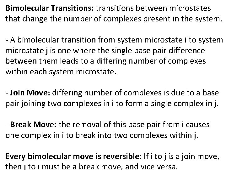
Bimolecular Transitions: transitions between microstates that change the number of complexes present in the system. - A bimolecular transition from system microstate i to system microstate j is one where the single base pair difference between them leads to a differing number of complexes within each system microstate. - Join Move: differing number of complexes is due to a base pair joining two complexes in i to form a single complex in j. - Break Move: the removal of this base pair from i causes one complex in i to break into two complexes within j. Every bimolecular move is reversible: If i to j is a join move, then j to i must be a break move, and vice versa.

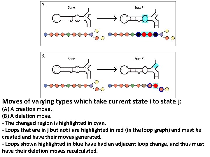
Moves of varying types which take current state i to state j: (A) A creation move. (B) A deletion move. - The changed region is highlighted in cyan. - Loops that are in j but not i are highlighted in red (in the loop graph) and must be created and have their moves generated. - Loops shown highlighted in blue have had an adjacent loop change, and thus must have their deletion moves recalculated.

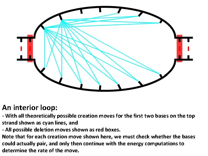
An interior loop: - With all theoretically possible creation moves for the first two bases on the top strand shown as cyan lines, and - All possible deletion moves shown as red boxes. Note that for each creation move shown here, we must check whether the bases could actually pair, and only then continue with the energy computations to determine the rate of the move.

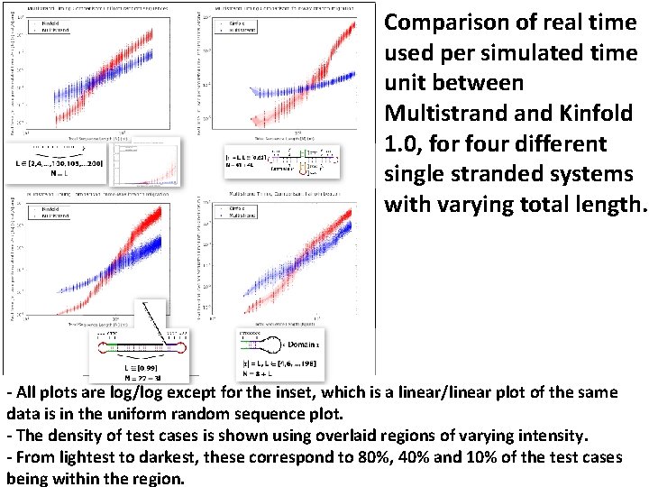
Comparison of real time used per simulated time unit between Multistrand Kinfold 1. 0, for four different single stranded systems with varying total length. - All plots are log/log except for the inset, which is a linear/linear plot of the same data is in the uniform random sequence plot. - The density of test cases is shown using overlaid regions of varying intensity. - From lightest to darkest, these correspond to 80%, 40% and 10% of the test cases being within the region.