The end of projective cameras Crossratios Twoview projective

The end of projective cameras • Cross-ratios • Two-view projective SFM • Multi-view geometry • More projective SFM Planches : – http: //www. di. ens. fr/~ponce/geomvis/lect 4. pptx – http: //www. di. ens. fr/~ponce/geomvis/lect 4. pdf

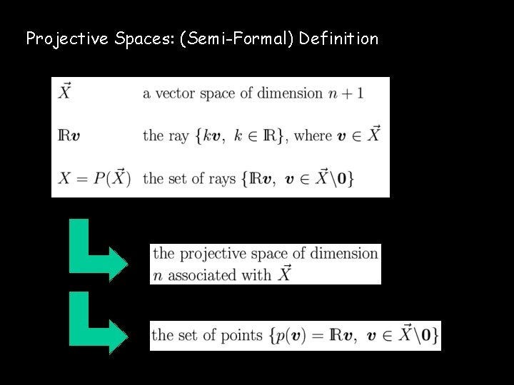
Projective Spaces: (Semi-Formal) Definition

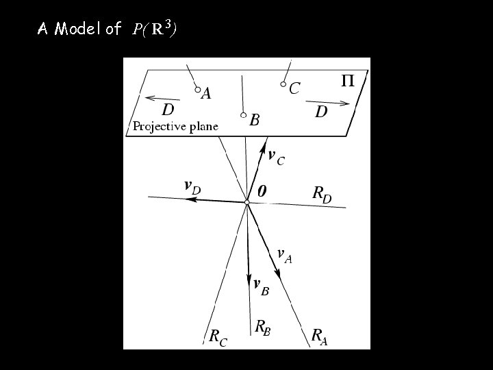
A Model of P( R 3)

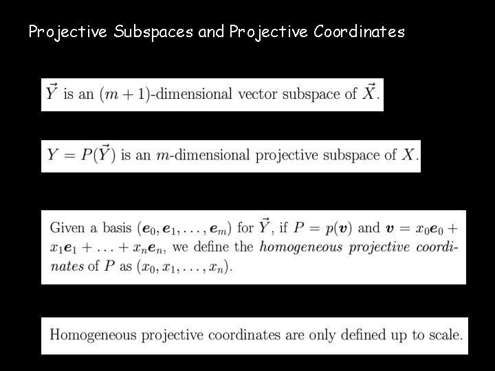
Projective Subspaces and Projective Coordinates

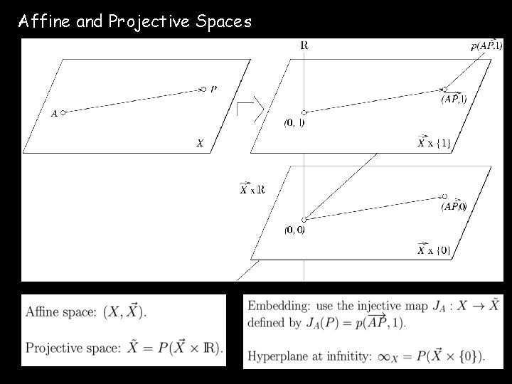
Affine and Projective Spaces

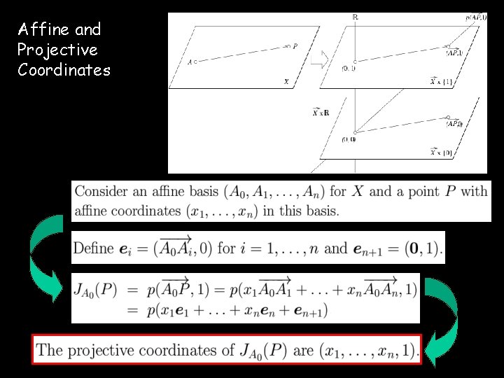
Affine and Projective Coordinates

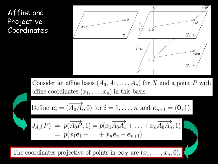
Affine and Projective Coordinates

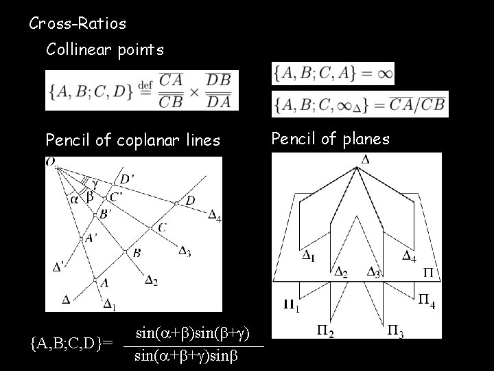
Cross-Ratios Collinear points Pencil of coplanar lines {A, B; C, D}= sin( + ) sin( + + )sin Pencil of planes

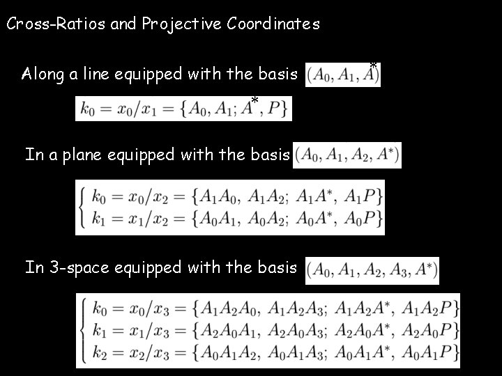
Cross-Ratios and Projective Coordinates * Along a line equipped with the basis In a plane equipped with the basis In 3 -space equipped with the basis * *

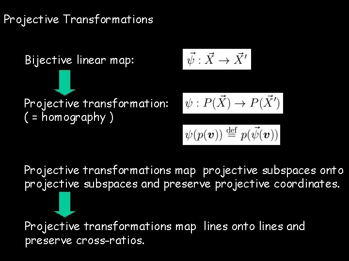
Projective Transformations Bijective linear map: Projective transformation: ( = homography ) Projective transformations map projective subspaces onto projective subspaces and preserve projective coordinates. Projective transformations map lines onto lines and preserve cross-ratios.

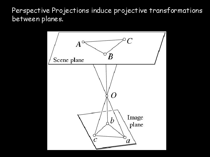
Perspective Projections induce projective transformations between planes.

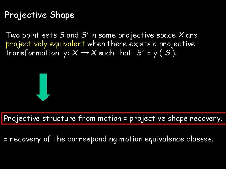
Projective Shape Two point sets S and S’ in some projective space X are projectively equivalent when there exists a projective transformation y: X X such that S’ = y ( S ). Projective structure from motion = projective shape recovery. = recovery of the corresponding motion equivalence classes.

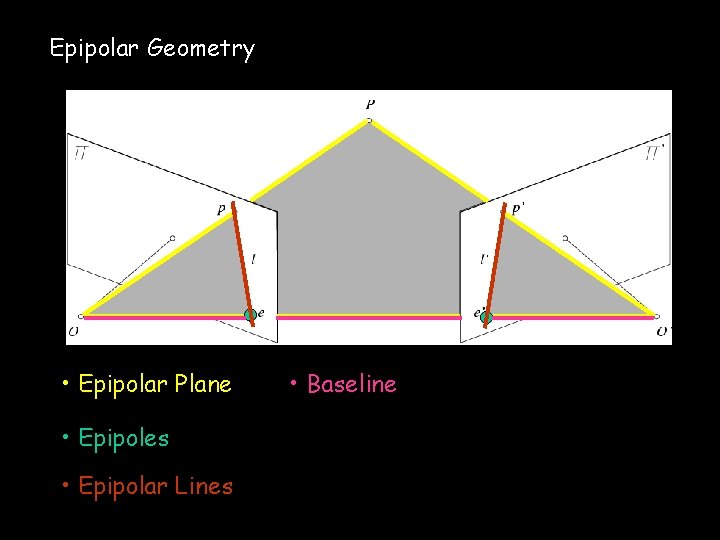
Epipolar Geometry • Epipolar Plane • Epipoles • Epipolar Lines • Baseline

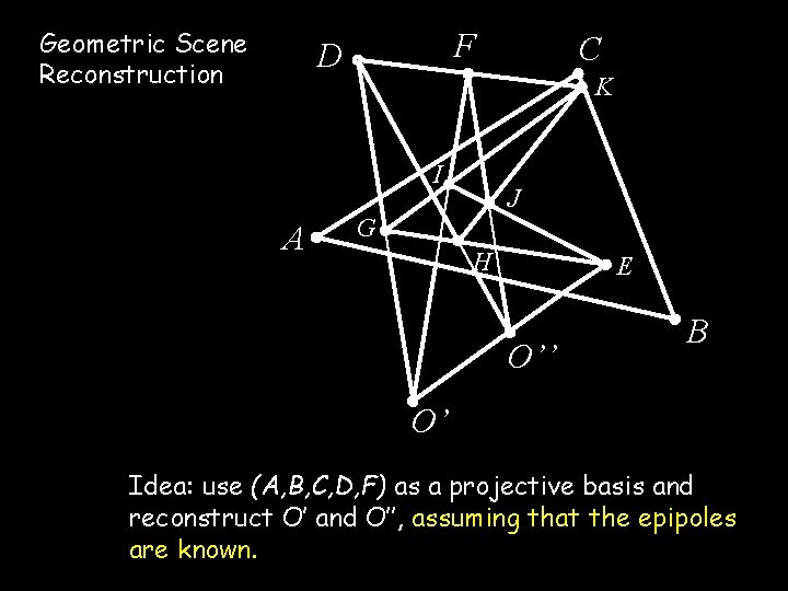
Geometric Scene Reconstruction F D K I A C J G H E O’’ B O’ Idea: use (A, B, C, D, F) as a projective basis and reconstruct O’ and O’’, assuming that the epipoles are known.

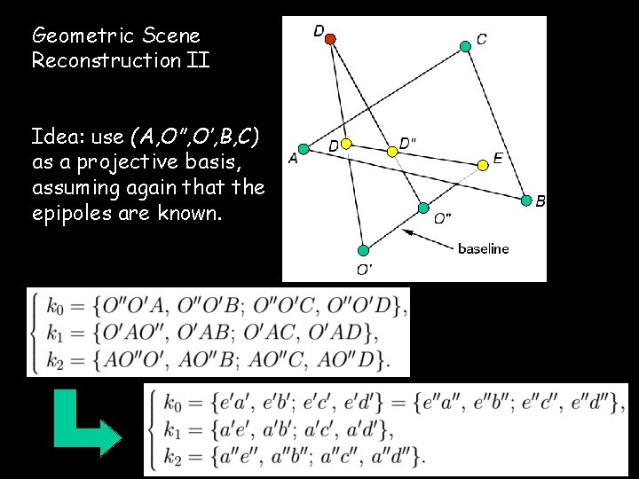
Geometric Scene Reconstruction II Idea: use (A, O”, O’, B, C) as a projective basis, assuming again that the epipoles are known.

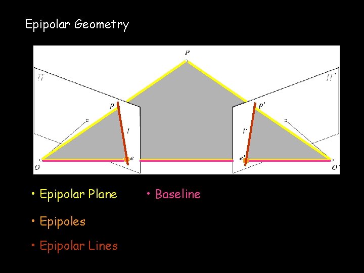
Epipolar Geometry • Epipolar Plane • Epipoles • Epipolar Lines • Baseline

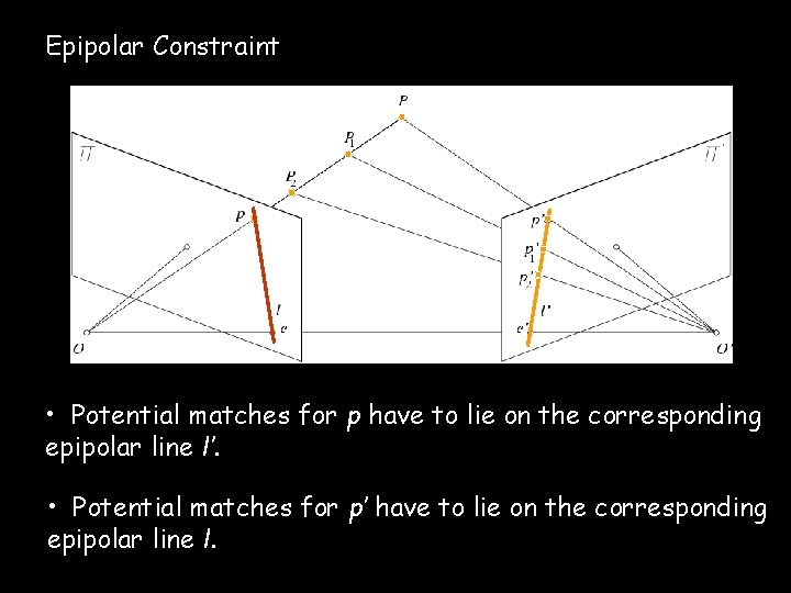
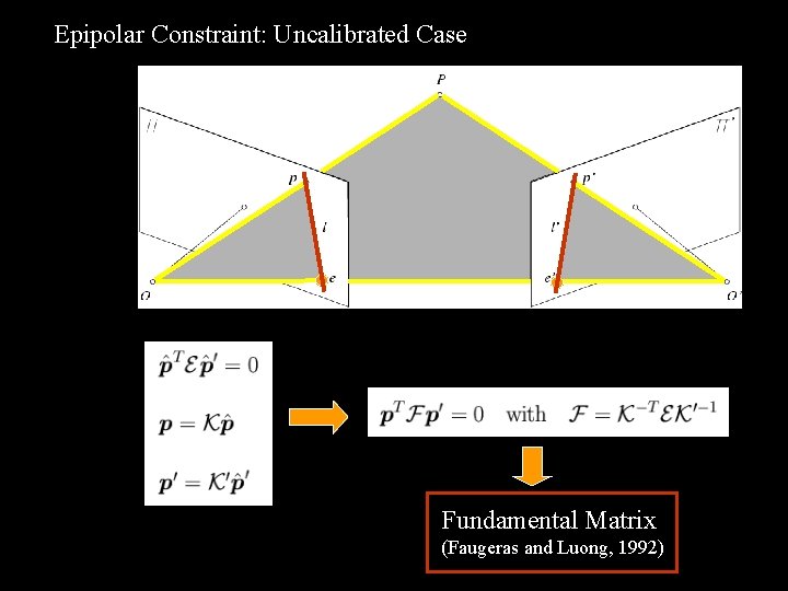
Epipolar Constraint • Potential matches for p have to lie on the corresponding epipolar line l’. • Potential matches for p’ have to lie on the corresponding epipolar line l.

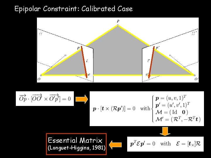
Epipolar Constraint: Calibrated Case Essential Matrix (Longuet-Higgins, 1981)

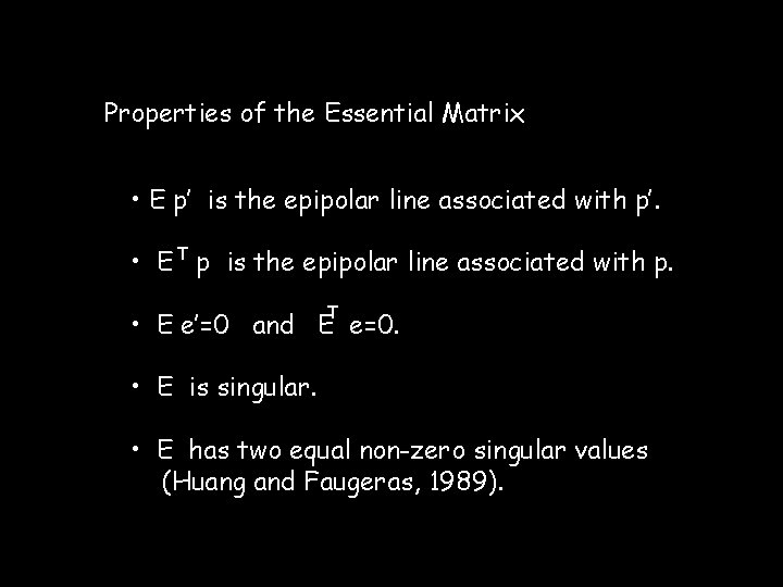
Properties of the Essential Matrix • E p’ is the epipolar line associated with p’. • E T p is the epipolar line associated with p. T • E e’=0 and E e=0. • E is singular. • E has two equal non-zero singular values (Huang and Faugeras, 1989).

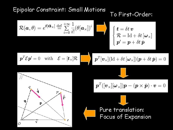
Epipolar Constraint: Small Motions To First-Order: Pure translation: Focus of Expansion

Epipolar Constraint: Uncalibrated Case Fundamental Matrix (Faugeras and Luong, 1992)

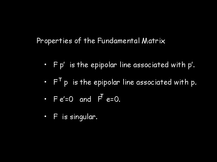
Properties of the Fundamental Matrix • F p’ is the epipolar line associated with p’. • F T p is the epipolar line associated with p. T • F e’=0 and F e=0. • F is singular.

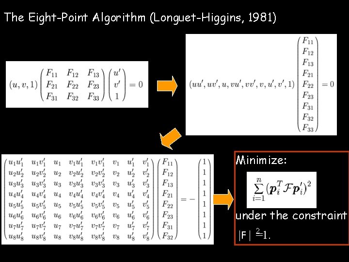
The Eight-Point Algorithm (Longuet-Higgins, 1981) Minimize: under the constraint 2 |F | =1.

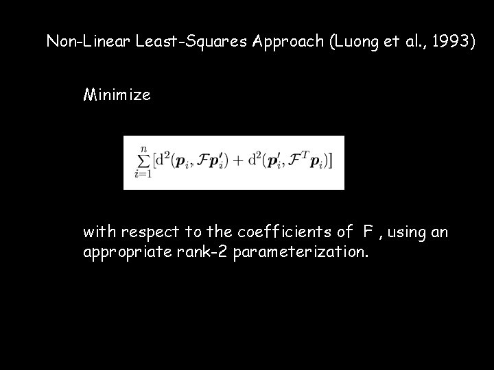
Non-Linear Least-Squares Approach (Luong et al. , 1993) Minimize with respect to the coefficients of F , using an appropriate rank-2 parameterization.

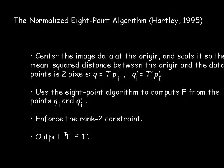
The Normalized Eight-Point Algorithm (Hartley, 1995) • Center the image data at the origin, and scale it so the mean squared distance between the origin and the data points is 2 pixels: q = T p , q’ = T’ p’. i i • Use the eight-point algorithm to compute F from the points q i and q’i. • Enforce the rank-2 constraint. • Output TT F T’.

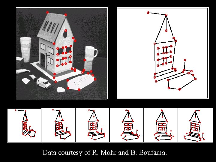
Data courtesy of R. Mohr and B. Boufama.

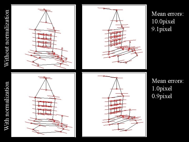
Without normalization With normalization Mean errors: 10. 0 pixel 9. 1 pixel Mean errors: 1. 0 pixel 0. 9 pixel