Projective cameras The end of projective SFM Euclidean

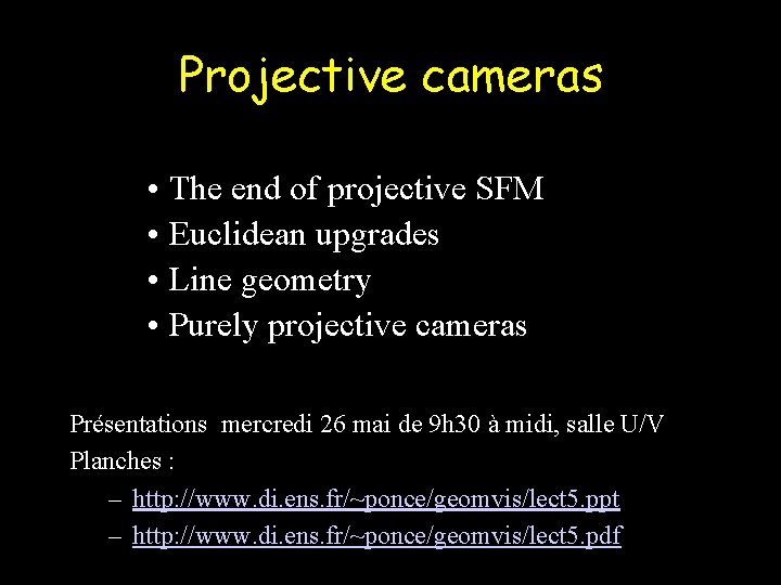
Projective cameras • The end of projective SFM • Euclidean upgrades • Line geometry • Purely projective cameras Présentations mercredi 26 mai de 9 h 30 à midi, salle U/V Planches : – http: //www. di. ens. fr/~ponce/geomvis/lect 5. ppt – http: //www. di. ens. fr/~ponce/geomvis/lect 5. pdf

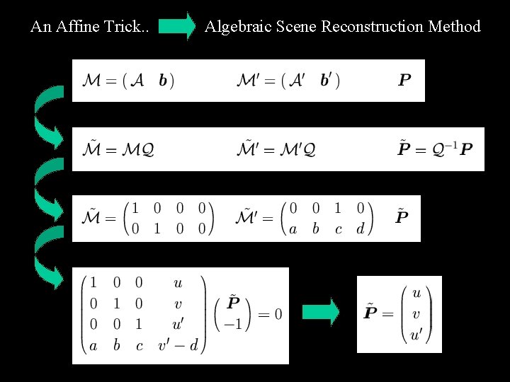
An Affine Trick. . Algebraic Scene Reconstruction Method

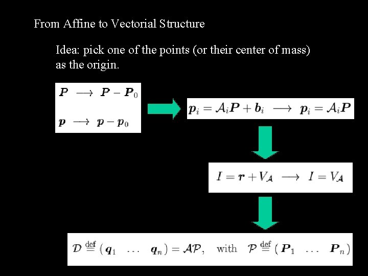
From Affine to Vectorial Structure Idea: pick one of the points (or their center of mass) as the origin.

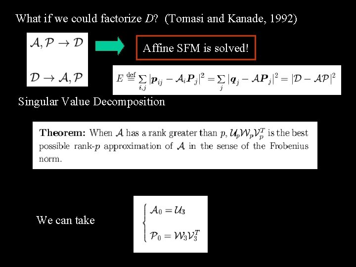
What if we could factorize D? (Tomasi and Kanade, 1992) Affine SFM is solved! Singular Value Decomposition We can take

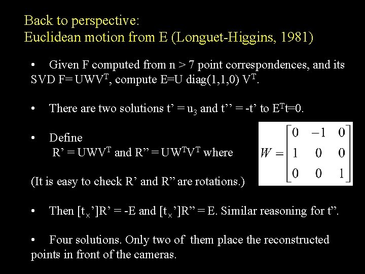
Back to perspective: Euclidean motion from E (Longuet-Higgins, 1981) • Given F computed from n > 7 point correspondences, and its SVD F= UWVT, compute E=U diag(1, 1, 0) VT. • There are two solutions t’ = u 3 and t’’ = -t’ to ETt=0. • Define R’ = UWVT and R” = UWTVT where (It is easy to check R’ and R” are rotations. ) • Then [t£’]R’ = -E and [t£’]R” = E. Similar reasoning for t”. • Four solutions. Only two of them place the reconstructed points in front of the cameras.

A different view of the fundamental matrix • Projective ambiguity ! M’Q=[Id 0] MQ=[A b]. • Hence: zp = [A b] P and z’p’ = [Id 0] P, with P=(x, y, z, 1)T. • This can be rewritten as: zp = ( A [Id 0] + [0 b] ) P = z’Ap’ + b. • Or: z (b £ p) = z’ (b £ Ap’). • Finally: p. TFp’ = 0 with F = [b£] A.

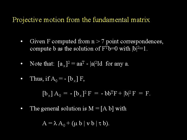
Projective motion from the fundamental matrix • Given F computed from n > 7 point correspondences, compute b as the solution of FTb=0 with |b|2=1. • Note that: [a£]2 = aa. T - |a|2 Id for any a. • Thus, if A 0 = - [b£] F, [b£] A 0 = - [b£]2 F = - bb. TF + |b|2 F = F. • The general solution is M = [A b] with A = A 0 + ( b | b).

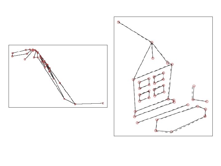
Two-view projective reconstruction. Mean relative error: 3. 0%

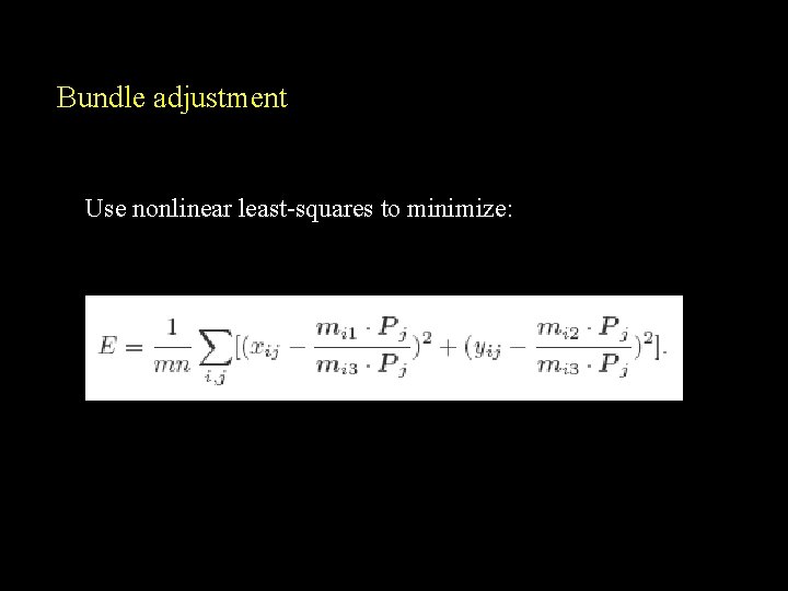
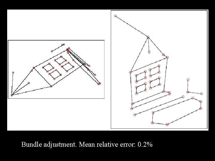
Bundle adjustment Use nonlinear least-squares to minimize:

Bundle adjustment. Mean relative error: 0. 2%

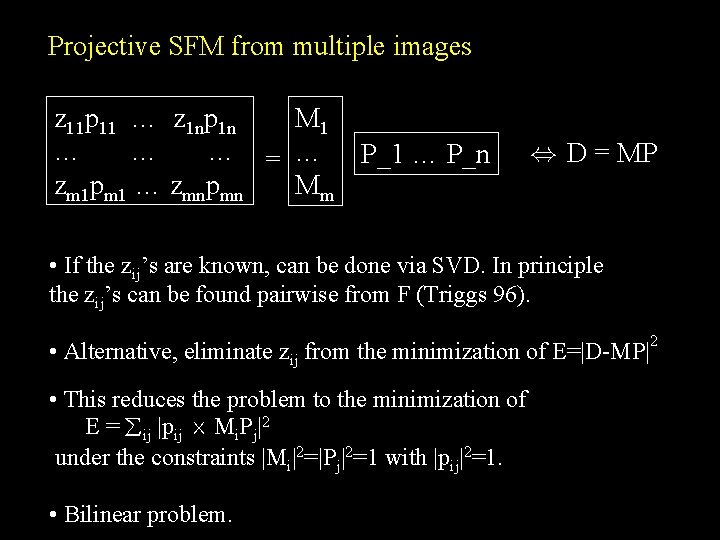
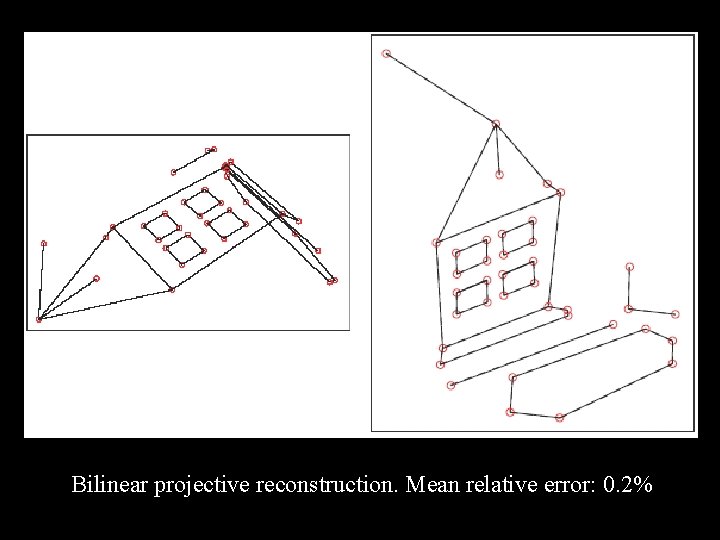
Projective SFM from multiple images z 11 p 11 … z 1 np 1 n M 1 … … … = … P_1 … P_n zm 1 pm 1 … zmnpmn Mm , D = MP • If the zij’s are known, can be done via SVD. In principle the zij’s can be found pairwise from F (Triggs 96). • Alternative, eliminate zij from the minimization of E=|D-MP| • This reduces the problem to the minimization of E = ij |pij £ Mi. Pj|2 under the constraints |Mi|2=|Pj|2=1 with |pij|2=1. • Bilinear problem. 2

Bilinear projective reconstruction. Mean relative error: 0. 2%

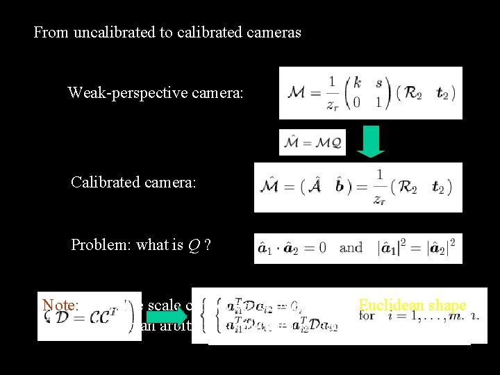
From uncalibrated to calibrated cameras Weak-perspective camera: Calibrated camera: Problem: what is Q ? Note: Absolute scale cannot be recovered. The Euclidean shape (defined up to an arbitrary similitude) is recovered.

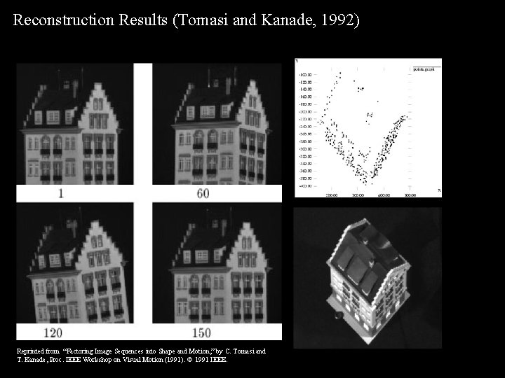
Reconstruction Results (Tomasi and Kanade, 1992) Reprinted from “Factoring Image Sequences into Shape and Motion, ” by C. Tomasi and T. Kanade, Proc. IEEE Workshop on Visual Motion (1991). 1991 IEEE.

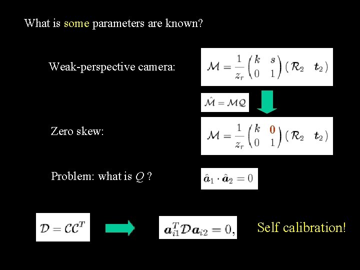
What is some parameters are known? Weak-perspective camera: Zero skew: 0 Problem: what is Q ? Self calibration!

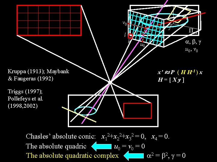
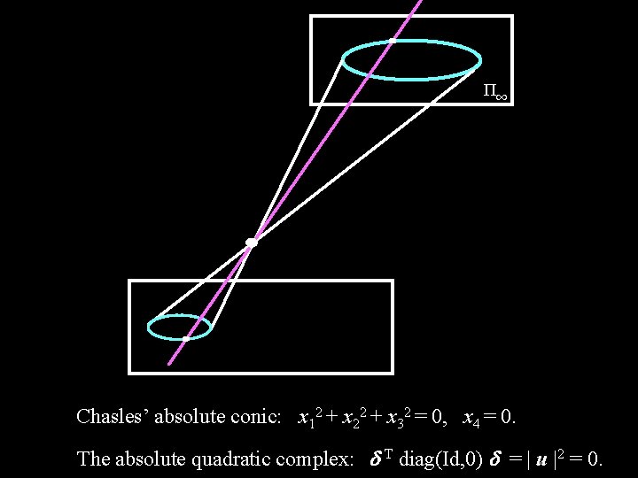
v 0 f l k Kruppa (1913); Maybank & Faugeras (1992) u 0 П 1 , , u 0, v 0 x’ ¼ P ( H H-1 ) x H=[Xy] Triggs (1997); Pollefeys et al. (1998, 2002) Chasles’ absolute conic: x 12+x 22+x 32 = 0, x 4 = 0. The absolute quadric u 0 = v 0 = 0 2 = 2, = 0 The absolute quadratic complex

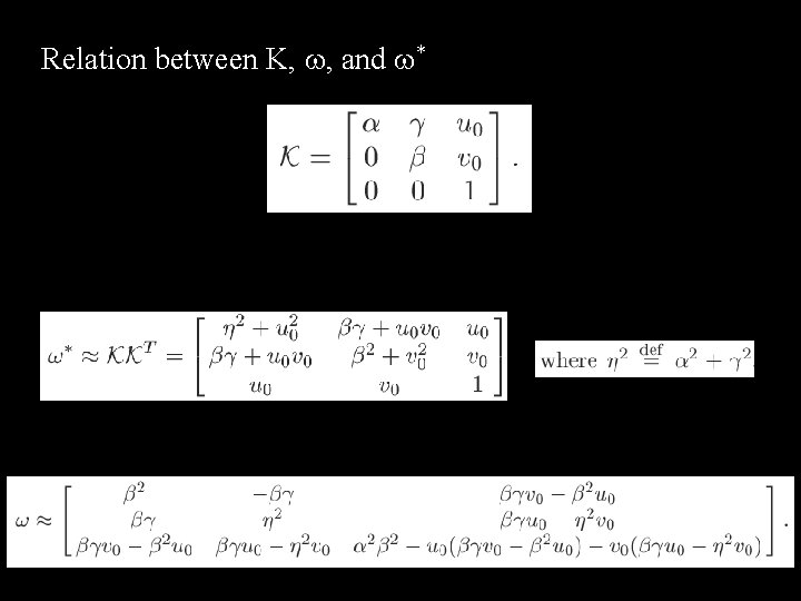
Relation between K, , and *

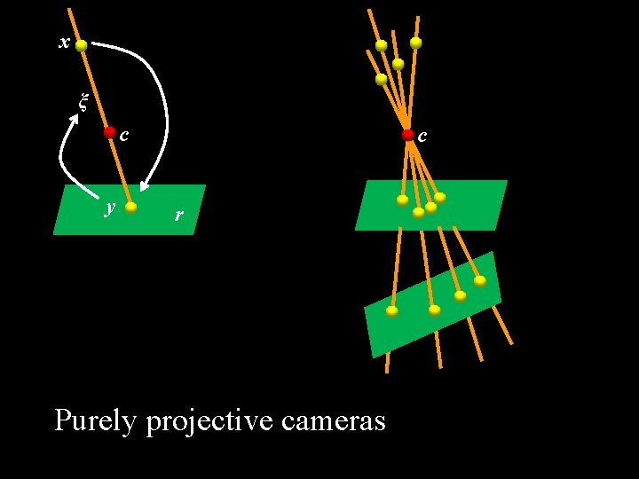
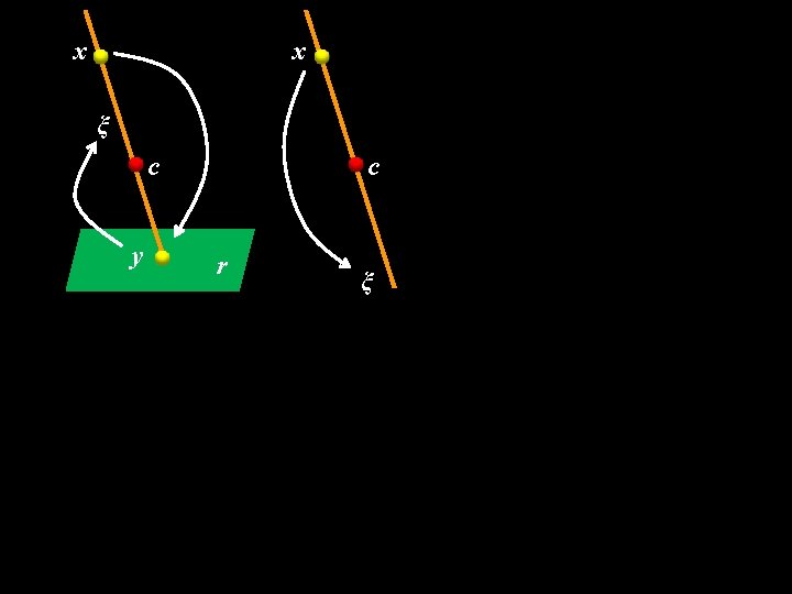
x ξ c y c r Purely projective cameras

x x ξ c y c r ξ

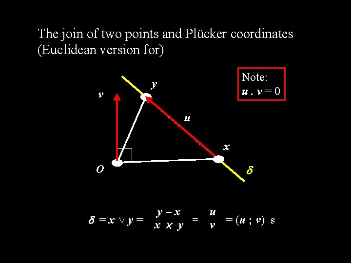
The join of two points and Plücker coordinates (Euclidean version for) v Note: u. v=0 y u x O y–x u = x Ç y = x £ y = v = (u ; v) s

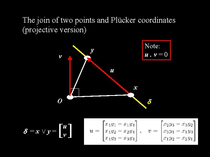
The join of two points and Plücker coordinates (projective version) v Note: u. v=0 y u x O [] u =xÇy= v

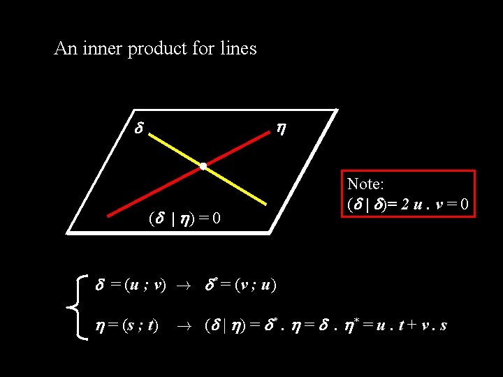
An inner product for lines ( | ) = 0 Note: ( | )= 2 u. v = 0 = (u ; v) ! * = (v ; u) = (s ; t) ! ( | ) = *. = . * = u. t + v. s

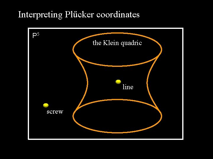
Interpreting Plűcker coordinates P 5 the Klein quadric line screw

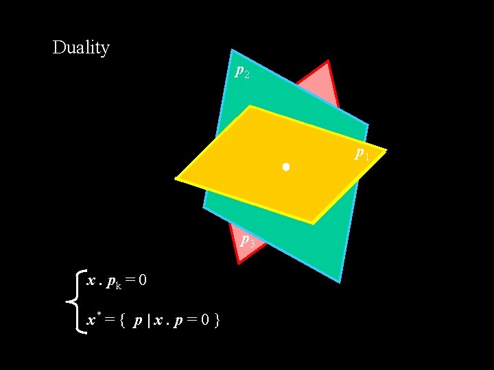
Duality p 2 p 1 x p 3 x. pk = 0 x* = { p | x. p = 0 }

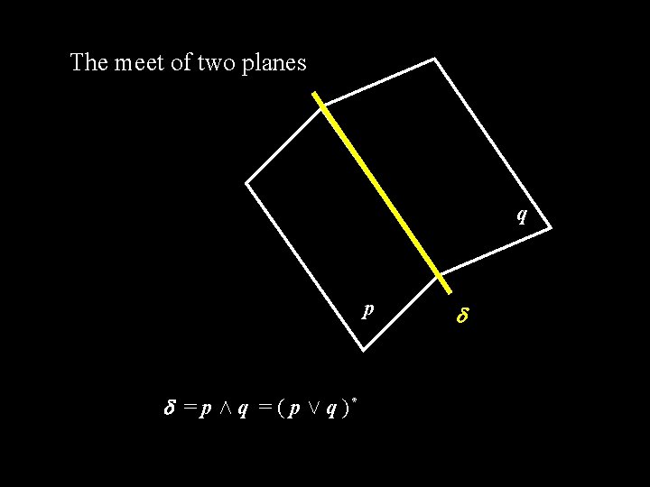
The meet of two planes q p = p Æ q = ( p Ç q )*

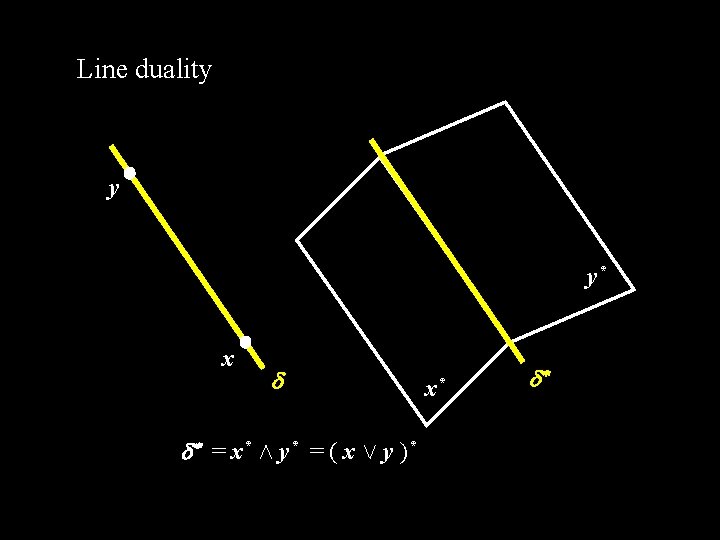
Line duality y y* x * = x* Æ y* = ( x Ç y )* x* *

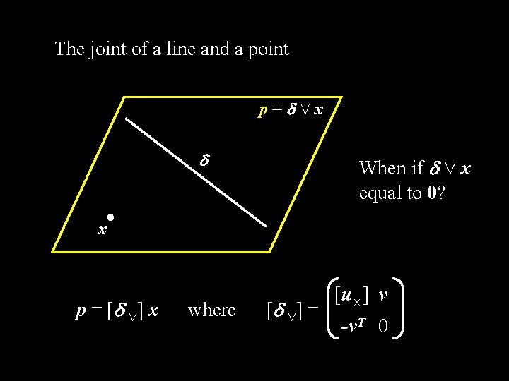
The joint of a line and a point p= Çx When if Ç x equal to 0? x p = [ Ç] x where [ Ç] = [u£] v -v. T 0

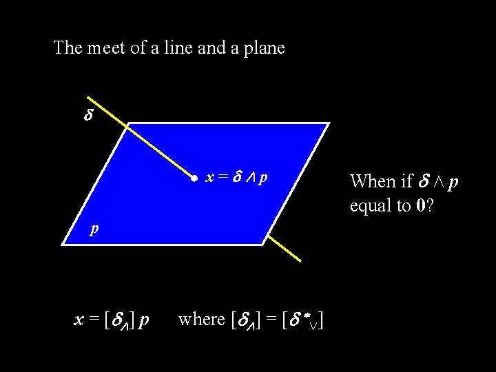
The meet of a line and a plane x= Æp p x = [ Æ] p where [ Æ] = [ *Ç] When if Æ p equal to 0?

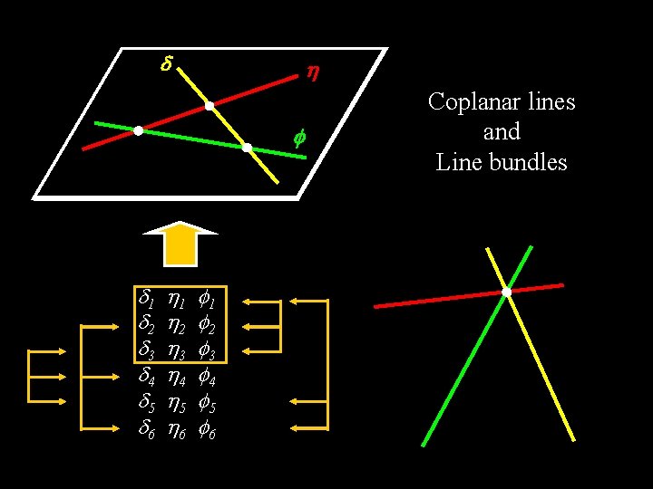
1 2 3 4 5 6 Coplanar lines and Line bundles

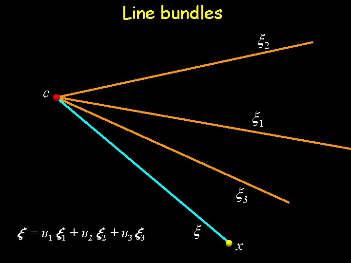
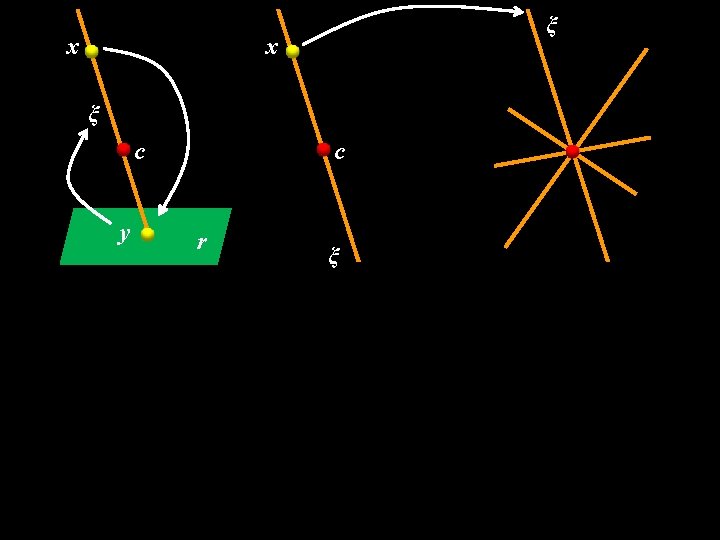
Line bundles x 2 c x 1 x 3 » = u 1 » 1 + u 2 » 2 + u 3 » 3 x x

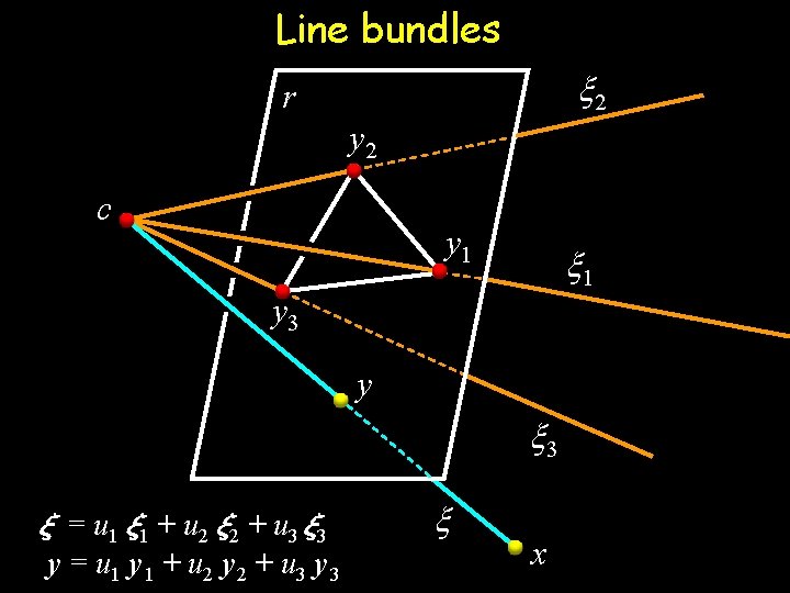
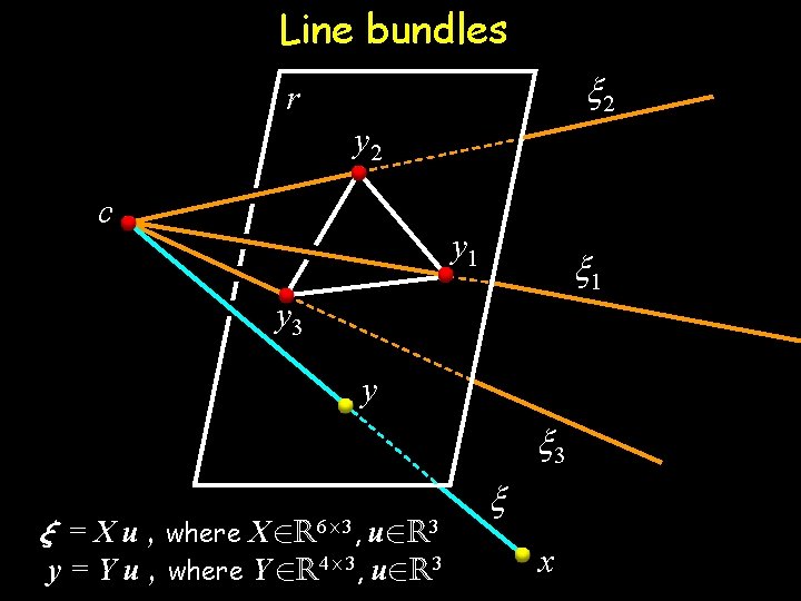
Line bundles x 2 r y 2 c y 1 x 1 y 3 y x 3 » = u 1 » 1 + u 2 » 2 + u 3 » 3 y = u 1 y 1 + u 2 y 2 + u 3 y 3 x x

Line bundles x 2 r y 2 c y 1 x 1 y 3 y x 3 » = X u , where X 2 R 6£ 3, u 2 R 3 y = Y u , where Y 2 R 4£ 3, u 2 R 3 x x

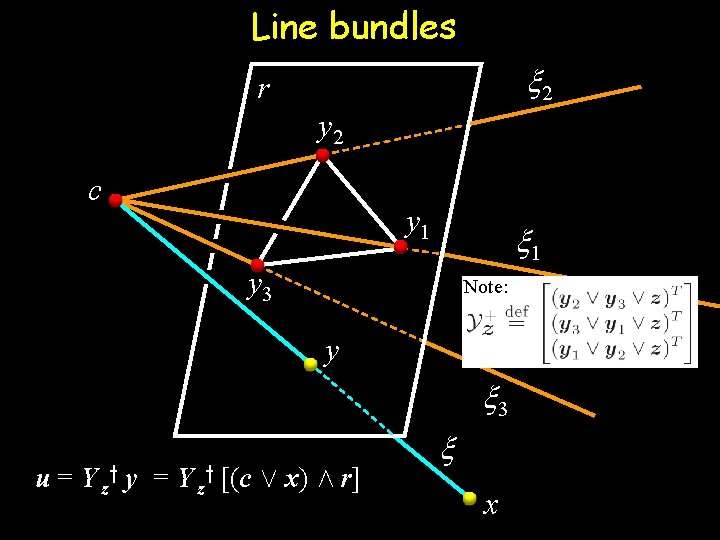
Line bundles x 2 r y 2 c y 1 x 1 y 3 Note: y x 3 u = Y z y y = Y z y [(c Ç x) Æ r] x x

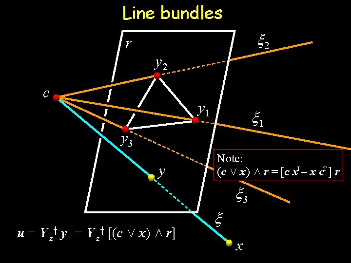
Line bundles x 2 r y 2 c y 1 x 1 y 3 y Note: (c Ç x) Æ r = [c x. T – x c. T ] r x 3 u = Y z y y = Y z y [(c Ç x) Æ r] x x

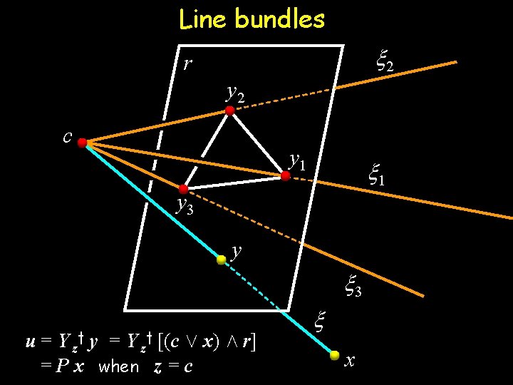
Line bundles x 2 r y 2 c y 1 x 1 y 3 y x 3 u = Y z y y = Y z y [(c Ç x) Æ r] = P x when z = c x x

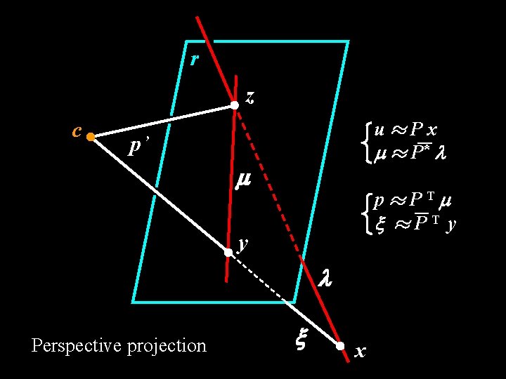
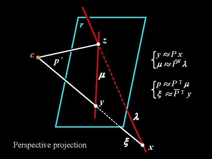
r z c u¼Px m ¼ P* l p’ m p¼PTm ¼PT y y l Perspective projection x

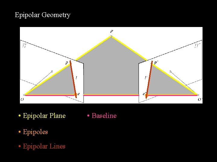
Epipolar Geometry • Epipolar Plane • Epipoles • Epipolar Lines • Baseline

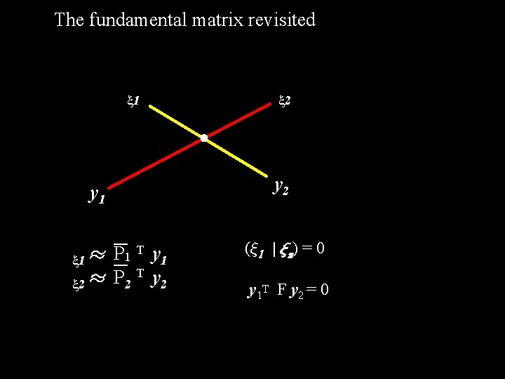
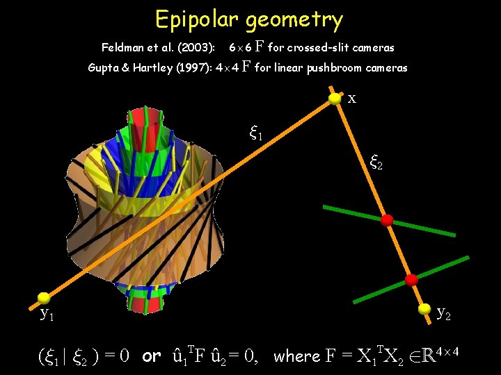
The fundamental matrix revisited x 1 y 1 T y ¼ P 1 1 x 1 T y ¼ P 2 2 x 2 y 2 (» 1 | » 2) = 0 y 1 T F y 2 = 0

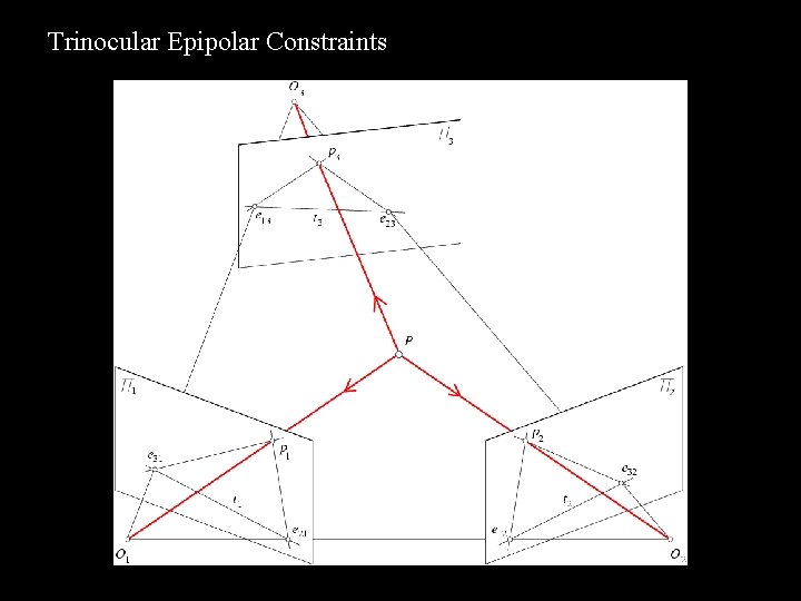
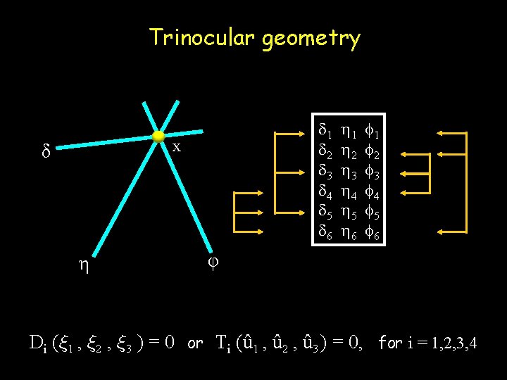
Trinocular Epipolar Constraints

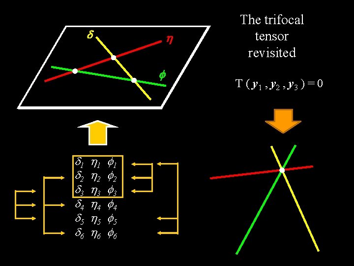
1 2 3 4 5 6 The trifocal tensor revisited T ( y 1 , y 2 , y 3 ) = 0

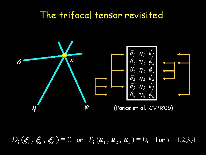
The trifocal tensor revisited 1 2 3 4 5 6 x δ η φ 1 2 3 4 5 6 (Ponce et al. , CVPR’ 05) Di (» 1 , » 2 , » 3 ) = 0 or T i (u 1 , u 2 , u 3 ) = 0, for i = 1, 2, 3, 4

r z c y¼Px m ¼ P* l p’ m p¼PTm ¼PT y y l Perspective projection x

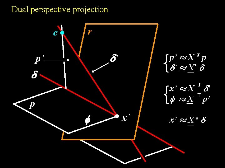
Dual perspective projection c r ’ p’ p’ ¼ X T p ’ ¼ X * x’ ¼ X ¼X p x’ T T ’ p’ x’ ¼ X*

П 1 Chasles’ absolute conic: x 12 + x 22 + x 32 = 0, x 4 = 0. The absolute quadratic complex: T diag(Id, 0) = | u |2 = 0.

Coordinate changes --- Metric upgrades x’ ¼ P ( H H-1 ) x H=[Xy] Planes: ep. T Points: ex Lines: e = H pp. T = H-1 px = p

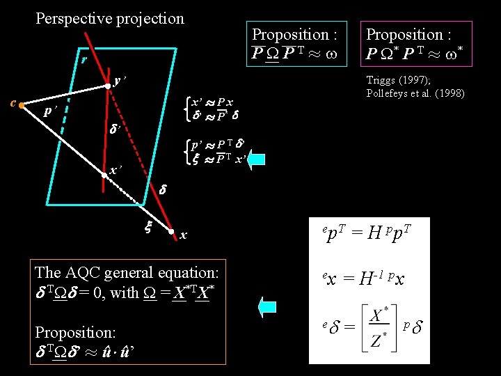
Perspective projection Proposition : P PT¼ r Proposition : P * P T ¼ * y’ c Triggs (1997); Pollefeys et al. (1998) x’ ¼ P x ’ ¼ P* p’ ’ p’ ¼ P T ’ ¼ P T x’ x’ x The AQC general equation: T = 0, with = X*TX* Proposition: T ’ ¼ û¢ û’ ep. T ex e = H pp. T = H-1 px = p

Relation between K, , and *

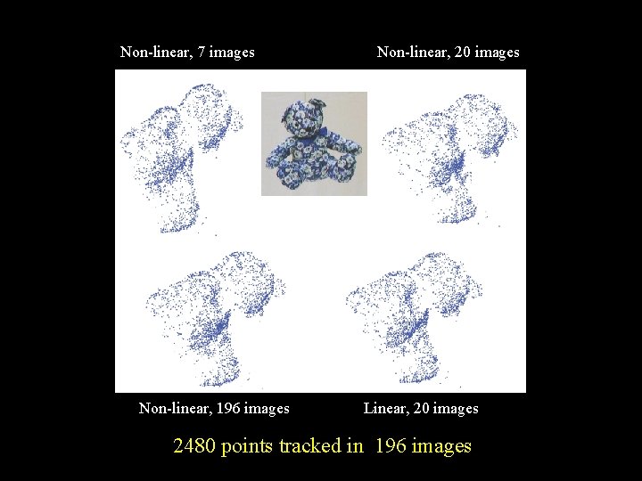
Non-linear, 7 images Non-linear, 196 images Non-linear, 20 images Linear, 20 images 2480 points tracked in 196 images

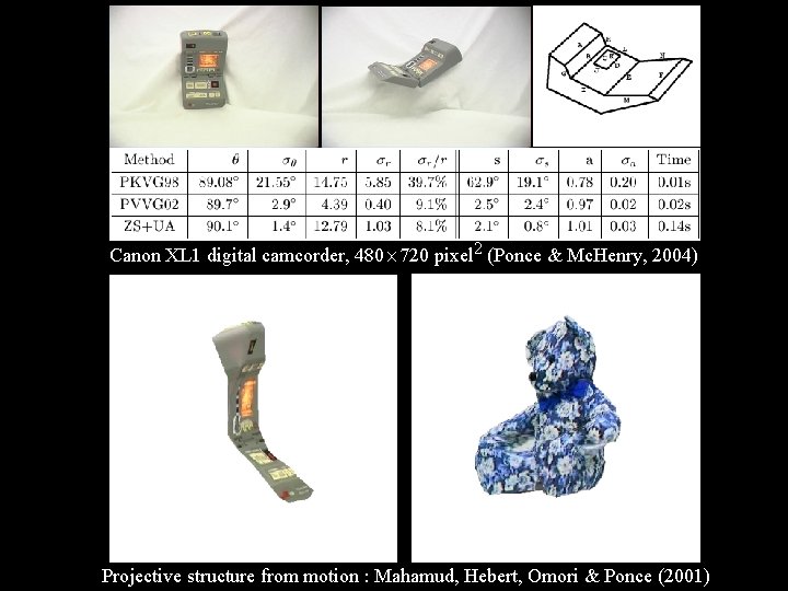
Canon XL 1 digital camcorder, 480£ 720 pixel 2 (Ponce & Mc. Henry, 2004) Projective structure from motion : Mahamud, Hebert, Omori & Ponce (2001)

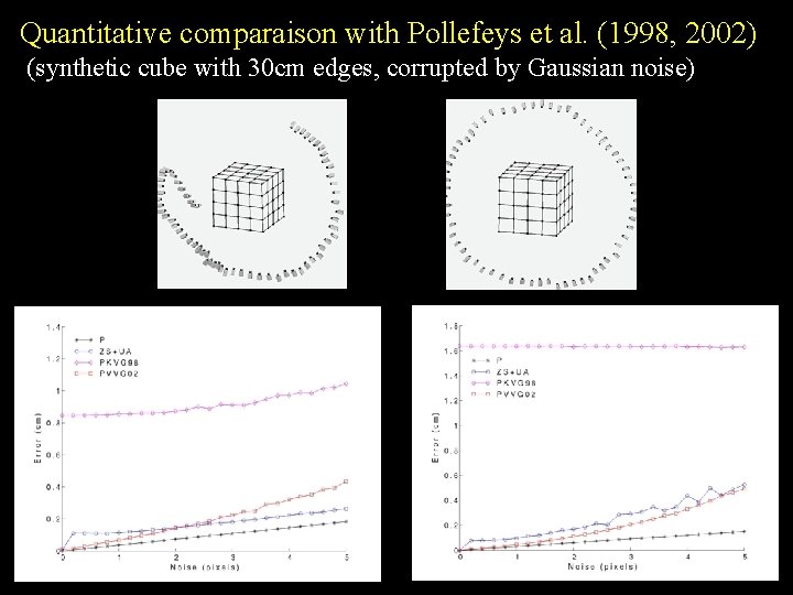
Quantitative comparaison with Pollefeys et al. (1998, 2002) (synthetic cube with 30 cm edges, corrupted by Gaussian noise)

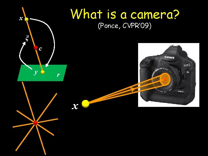
What is a camera? x (Ponce, CVPR’ 09) ξ c y r x

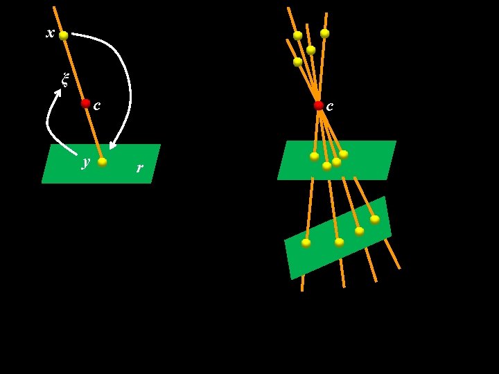
x ξ c y c r

x x ξ c y c r ξ

x ξ c y c r ξ

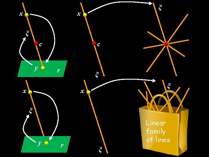
x ξ c y c r ξ x ξ y r Linear family of lines ξ

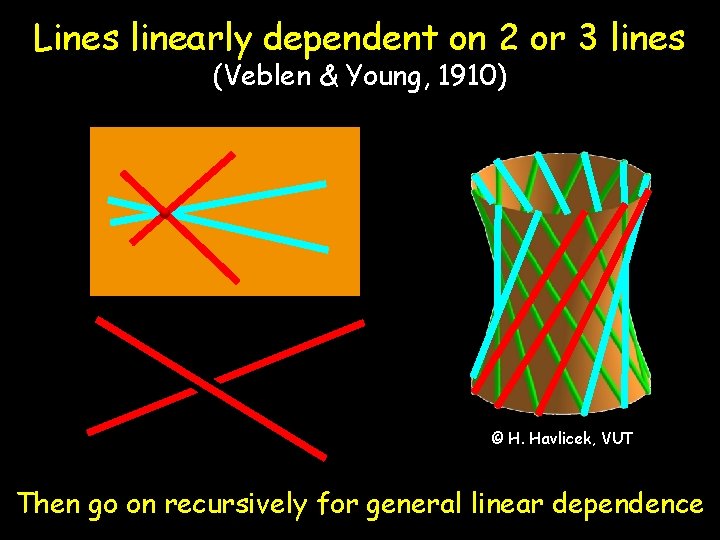
Lines linearly dependent on 2 or 3 lines (Veblen & Young, 1910) © H. Havlicek, VUT Then go on recursively for general linear dependence

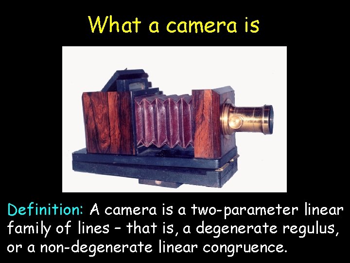
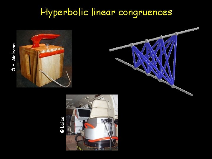
What a camera is Definition: A camera is a two-parameter linear family of lines – that is, a degenerate regulus, or a non-degenerate linear congruence.

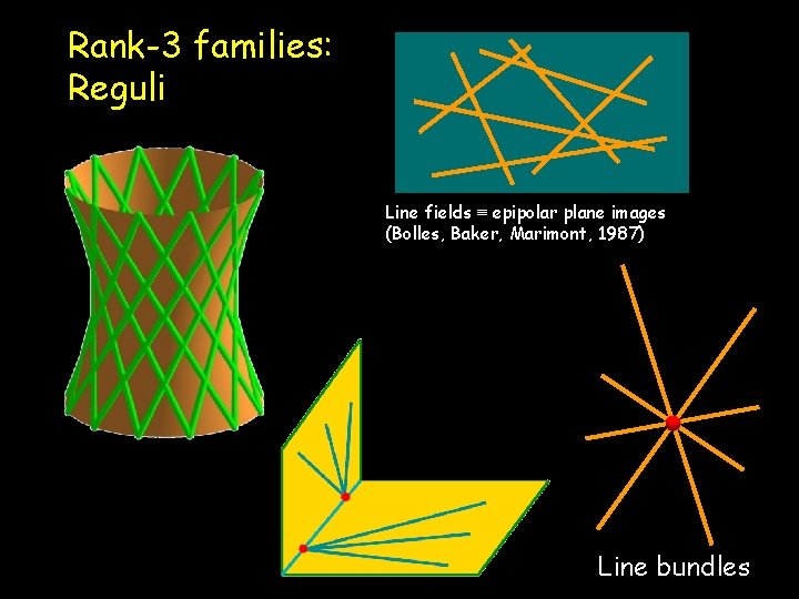
Rank-3 families: Reguli Line fields ≡ epipolar plane images (Bolles, Baker, Marimont, 1987) Line bundles

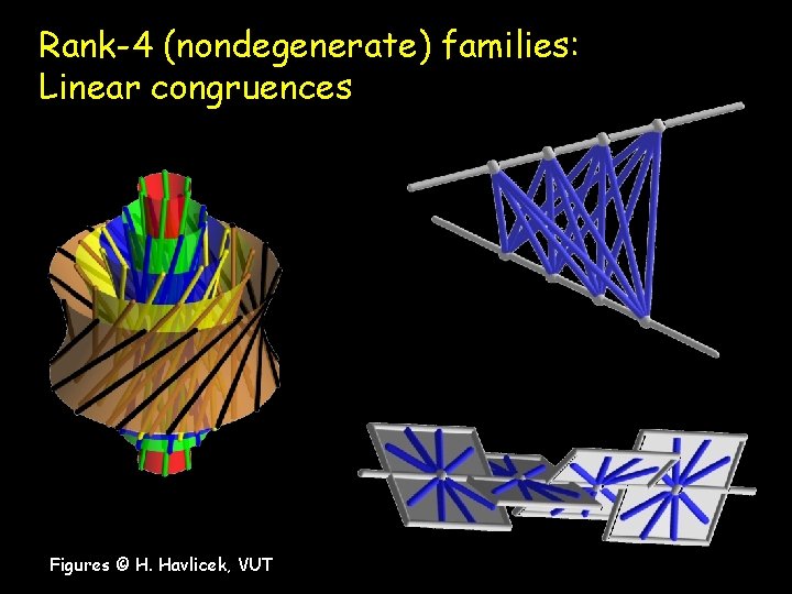
Rank-4 (nondegenerate) families: Linear congruences Figures © H. Havlicek, VUT

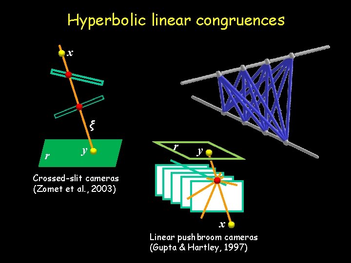
Hyperbolic linear congruences x ξ r y Crossed-slit cameras (Zomet et al. , 2003) ξ x Linear pushbroom cameras (Gupta & Hartley, 1997)

© Leica © E. Molzcan Hyperbolic linear congruences

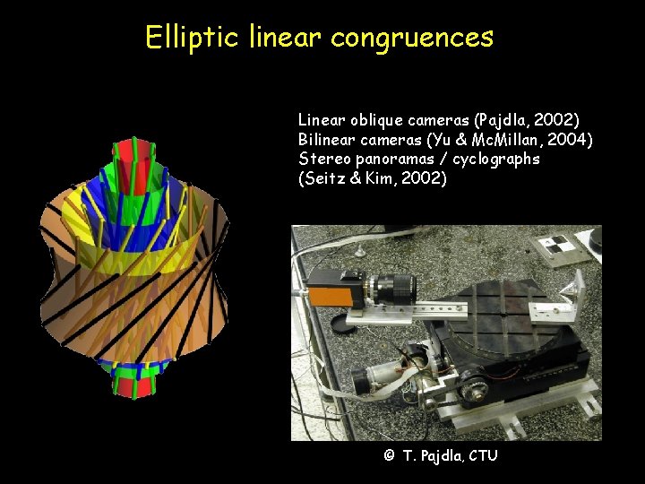
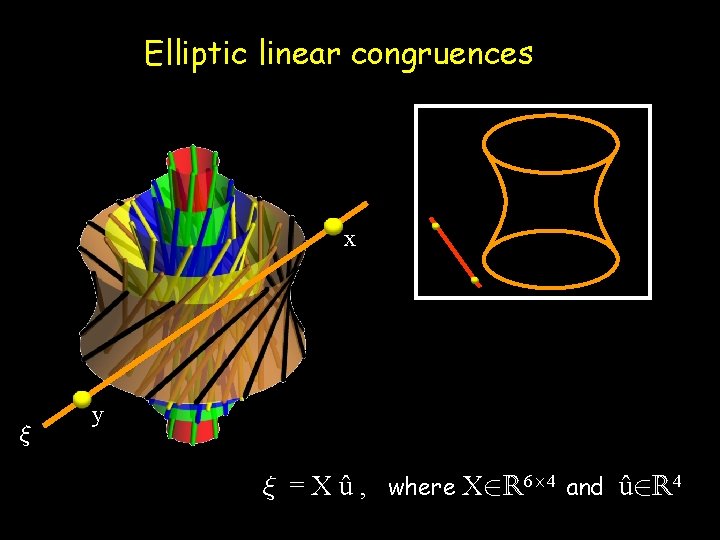
Elliptic linear congruences Linear oblique cameras (Pajdla, 2002) Bilinear cameras (Yu & Mc. Millan, 2004) Stereo panoramas / cyclographs (Seitz & Kim, 2002) © T. Pajdla, CTU

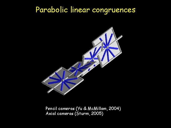
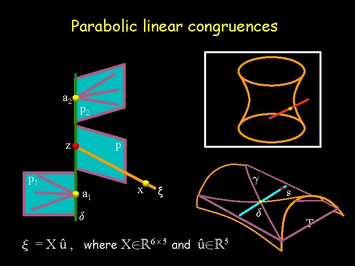
Parabolic linear congruences Pencil cameras (Yu & Mc. Millam, 2004) Axial cameras (Sturm, 2005)

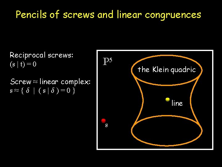
Plücker coordinates and the Klein quadric x Note: y [] P 5 u =xÇy= v u. v=0 the Klein quadric line screw

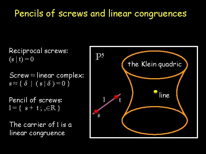
Pencils of screws and linear congruences Reciprocal screws: (s | t) = 0 P 5 the Klein quadric Screw ≈ linear complex: s≈{± | (s|±)=0} line s

Pencils of screws and linear congruences Reciprocal screws: (s | t) = 0 P 5 the Klein quadric Screw ≈ linear complex: s≈{± | (s|±)=0} Pencil of screws: l = { s + t ; , 2 R } The carrier of l is a linear congruence l s t line

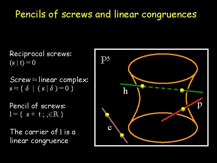
Pencils of screws and linear congruences Reciprocal screws: (s | t) = 0 P 5 Screw ≈ linear complex: s≈{± | (s|±)=0} h p Pencil of screws: l = { s + t ; , 2 R } The carrier of l is a linear congruence e

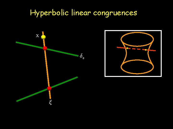
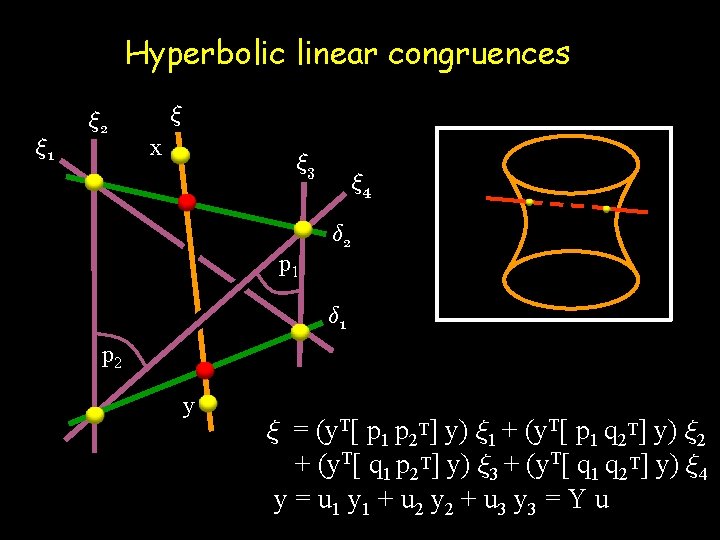
Hyperbolic linear congruences x ± 2 »

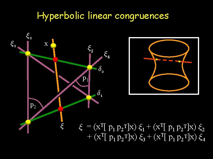
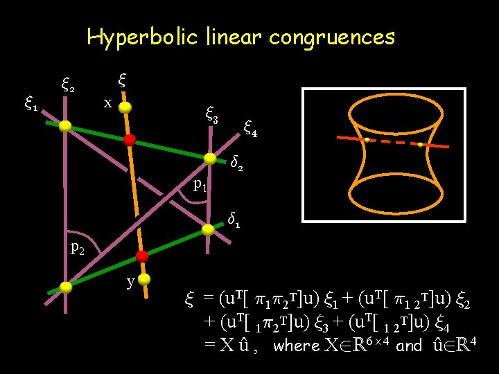
Hyperbolic linear congruences » 1 » 2 x » 3 p 1 » 4 ± 2 ± 1 p 2 » » = (x. T[ p 1 p 2 T]x) » 1 + (x. T[ p 1 p 2 T]x) » 2 + (x. T[ p 1 p 2 T]x) » 3 + (x. T[ p 1 p 2 T]x) » 4

Hyperbolic linear congruences » 1 » 2 » x » 3 p 1 » 4 ± 2 ± 1 p 2 y » = (y. T[ p 1 p 2 T] y) » 1 + (y. T[ p 1 q 2 T] y) » 2 + (y. T[ q 1 p 2 T] y) » 3 + (y. T[ q 1 q 2 T] y) » 4 y = u 1 y 1 + u 2 y 2 + u 3 y 3 = Y u

Hyperbolic linear congruences » 1 » 2 » x » 3 p 1 » 4 ± 2 ± 1 p 2 y » = (u. T[ ¼ 1¼ 2 T]u) » 1 + (u. T[ ¼ 1 2 T]u) » 2 + (u. T[ 1¼ 2 T]u) » 3 + (u. T[ 1 2 T]u) » 4 = X û , where X 2 R 6£ 4 and û 2 R 4

Parabolic linear congruences a 2 p z p 1 a 1 x ξ ± » = X û , where X 2 R 6£ 5 and û 2 R 5 ° s ± T

Elliptic linear congruences x » y » = X û , where X 2 R 6£ 4 and û 2 R 4

Epipolar geometry Feldman et al. (2003): 6£ 6 F for crossed-slit cameras Gupta & Hartley (1997): 4£ 4 F for linear pushbroom cameras x » 1 » 2 y 1 (» 1 | » 2 ) = 0 or û F û 2 = 0, where F = X 1 X 2 2 R 4£ 4 T 1 T

Trinocular geometry 1 2 3 4 5 6 x δ η 1 2 3 4 5 6 φ Di (» 1 , » 2 , » 3 ) = 0 or Ti (û 1 , û 2 , û 3 ) = 0, for i = 1, 2, 3, 4

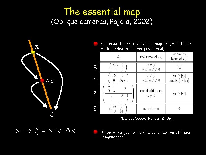
The essential map (Oblique cameras, Pajdla, 2002) Canonical forms of essential maps A ( = matrices with quadratic minimal poylnomial) x B Ax H P ξ x ! ξ = x Ç Ax E (Batog, Goaoc, Ponce, 2009) Alternative geometric characterization of linear congruences

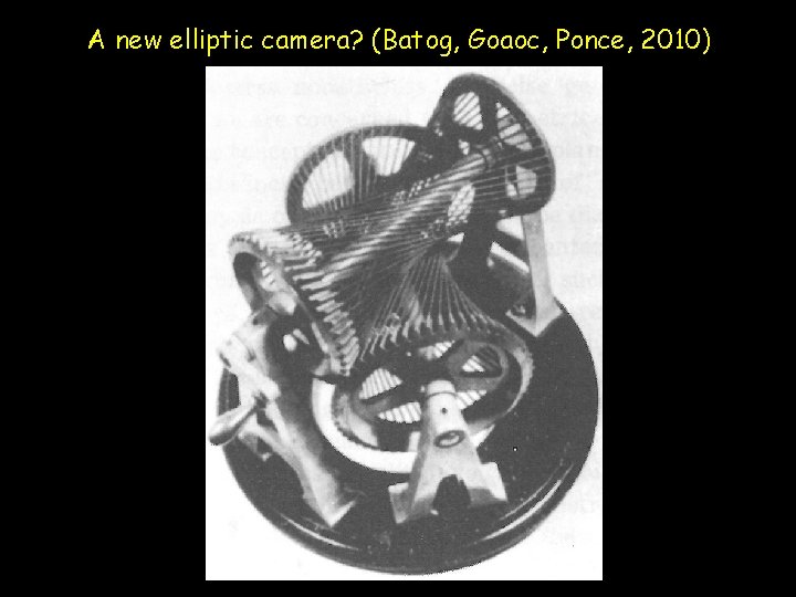
A new elliptic camera? (Batog, Goaoc, Ponce, 2010)