System Identification CSE 421 Digital Control Lecture 12

System Identification CSE 421 Digital Control Lecture 12 1

Introduction • In order to be able to design a controller for a dynamic system, we must have a model of the system describing its dynamic behavior. • In principle, there are two approaches to finding the model: physical modeling and system identification. • Physical modeling is analytical approach in which basic principles (laws of motion, electrical laws, …) are used to obtains di�erential equations describing system behavior. • While this is useful in gaining insight into system behavior, actual physical phenomena may be too complex to permit satisfactory description using physical principles. 2

System identification • When physical modeling is not feasible, we may resort to the experimental approach called system identification. • In this approach, we first excite the plant with some input sequence, u(0), u(1), …, u(N), and record the corresponding output response, y(0), y(1), …, y(N). Then, we construct a model from this observed data. • In these slides, a brief introduction to system identification using the least squares method is presented. 3

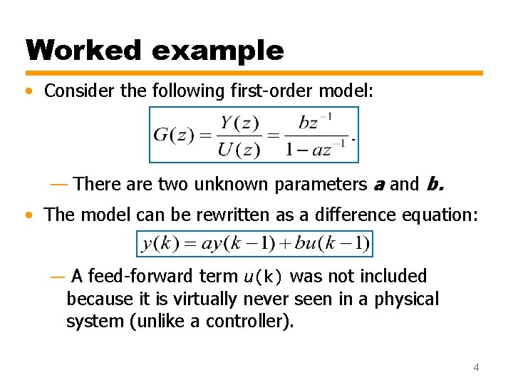
Worked example • Consider the following first-order model: — There are two unknown parameters a and b. • The model can be rewritten as a difference equation: — A feed-forward term u(k) was not included because it is virtually never seen in a physical system (unlike a controller). 4

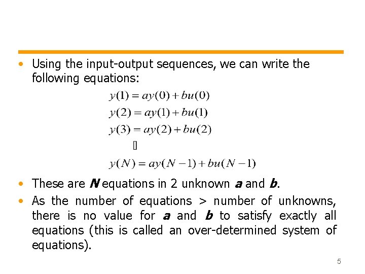
• Using the input-output sequences, we can write the following equations: • These are N equations in 2 unknown a and b. • As the number of equations > number of unknowns, there is no value for a and b to satisfy exactly all equations (this is called an over-determined system of equations). 5

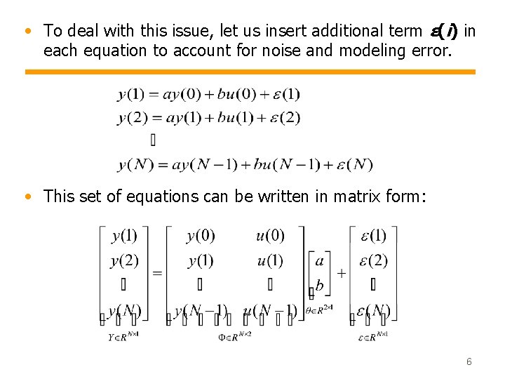
• To deal with this issue, let us insert additional term ε(i) in each equation to account for noise and modeling error. • This set of equations can be written in matrix form: 6

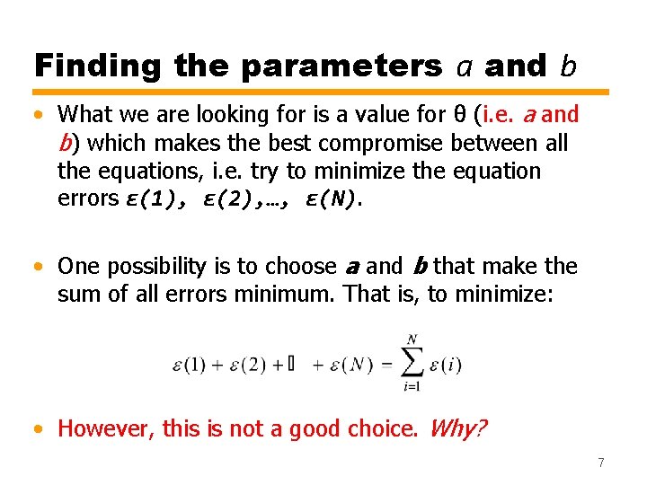
Finding the parameters a and b • What we are looking for is a value for θ (i. e. a and b) which makes the best compromise between all the equations, i. e. try to minimize the equation errors ε(1), ε(2), …, ε(N). • One possibility is to choose a and b that make the sum of all errors minimum. That is, to minimize: • However, this is not a good choice. Why? 7

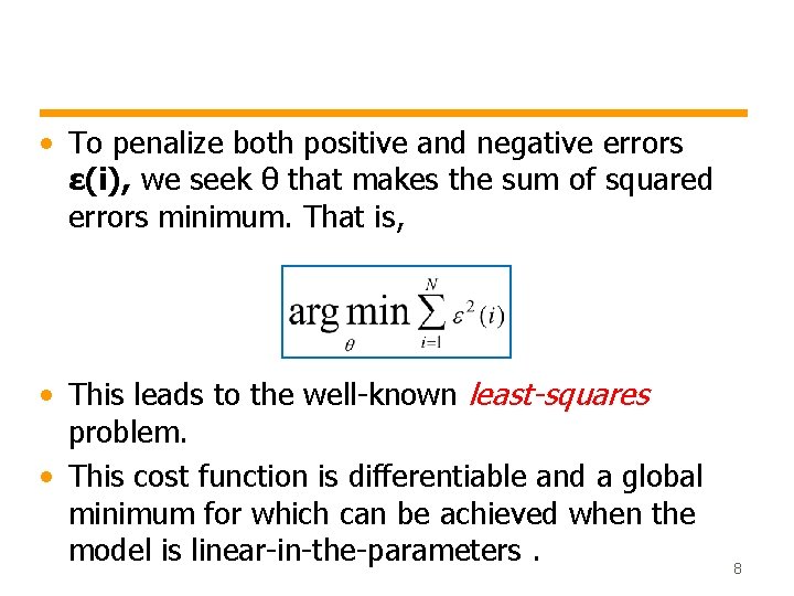
• To penalize both positive and negative errors ε(i), we seek θ that makes the sum of squared errors minimum. That is, • This leads to the well-known least-squares problem. • This cost function is differentiable and a global minimum for which can be achieved when the model is linear-in-the-parameters. 8

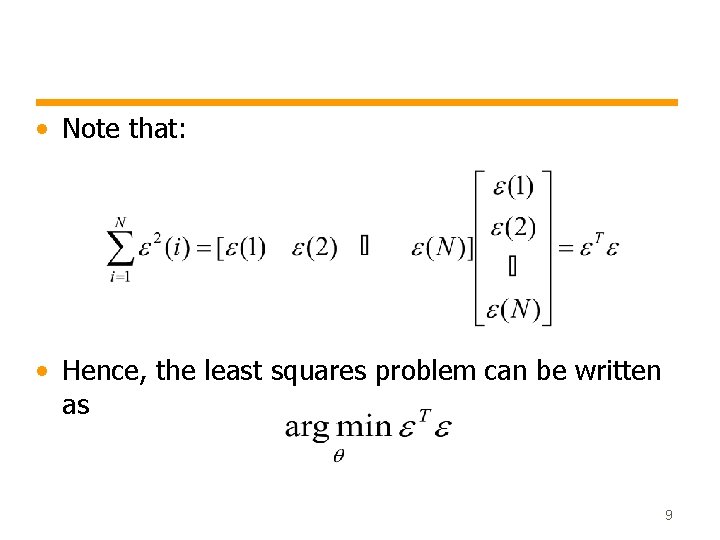
• Note that: • Hence, the least squares problem can be written as 9

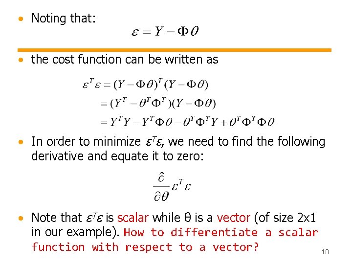
• Noting that: • the cost function can be written as • In order to minimize εTε, we need to find the following derivative and equate it to zero: • Note that εTε is scalar while θ is a vector (of size 2 x 1 in our example). How to differentiate a scalar function with respect to a vector? 10

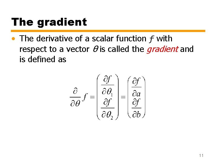
The gradient • The derivative of a scalar function f with respect to a vector θ is called the gradient and is defined as 11

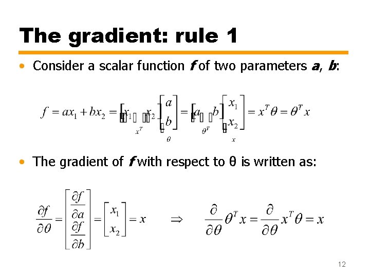
The gradient: rule 1 • Consider a scalar function f of two parameters a, b: • The gradient of f with respect to θ is written as: 12

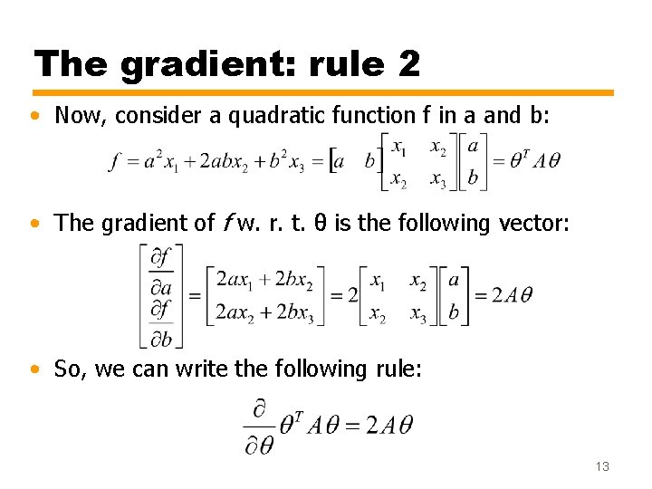
The gradient: rule 2 • Now, consider a quadratic function f in a and b: • The gradient of f w. r. t. θ is the following vector: • So, we can write the following rule: 13

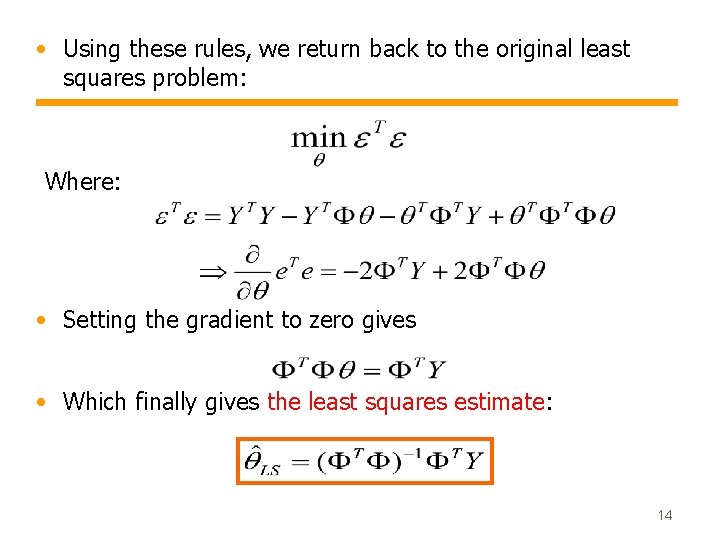
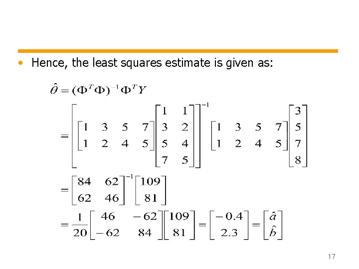
• Using these rules, we return back to the original least squares problem: Where: • Setting the gradient to zero gives • Which finally gives the least squares estimate: 14

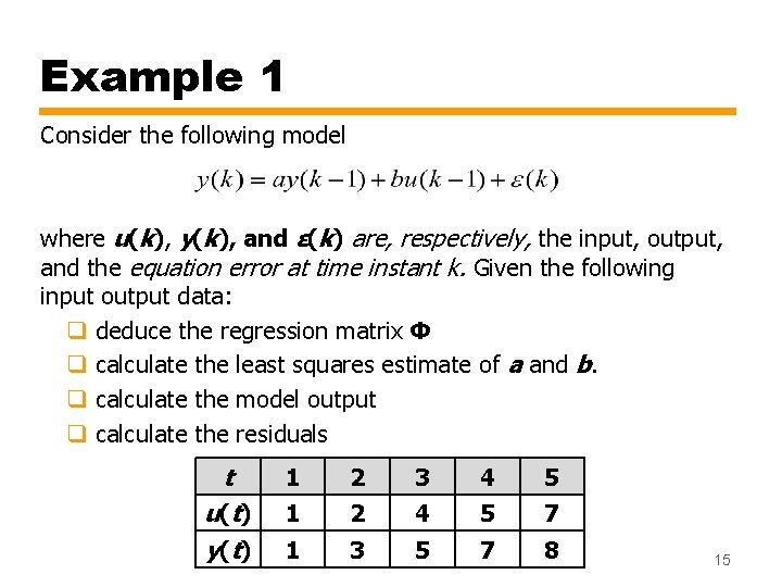
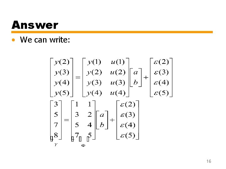
Example 1 Consider the following model where u(k), y(k), and ε(k) are, respectively, the input, output, and the equation error at time instant k. Given the following input output data: q deduce the regression matrix Φ q calculate the least squares estimate of a and b. q calculate the model output q calculate the residuals t u (t ) y (t ) 1 2 3 4 5 1 2 4 5 7 1 3 5 7 8 15

Answer • We can write: 16

• Hence, the least squares estimate is given as: 17

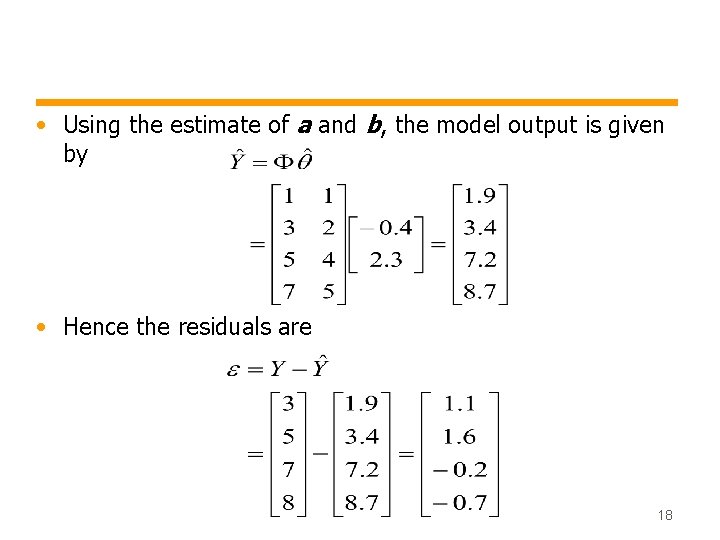
• Using the estimate of a and b, the model output is given by • Hence the residuals are 18

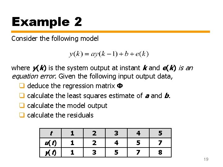
Example 2 Consider the following model where y(k) is the system output at instant k and e(k) is an equation error. Given the following input output data, q deduce the regression matrix Φ q calculate the least squares estimate of a and b. q calculate the model output q calculate the residuals t u (t ) y (t ) 1 2 3 4 5 1 2 4 5 7 1 3 5 7 8 19

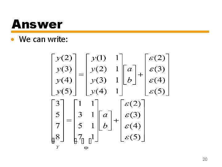
Answer • We can write: 20

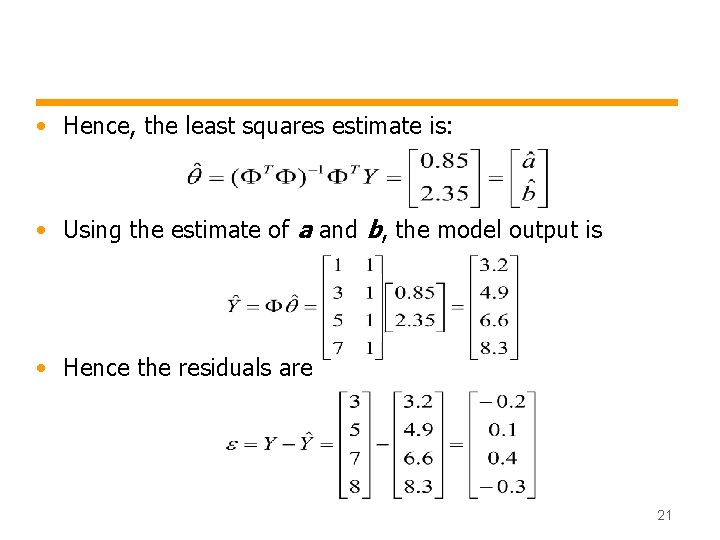
• Hence, the least squares estimate is: • Using the estimate of a and b, the model output is • Hence the residuals are 21

Model order selection • The choice of model order (i. e. the number of parameters) is up to the designer. • The designer may perform multiple fits with di�erent orders and select the lowest order fit that yields acceptable agreement. • Selecting a model of too-high order means that you use the “extra” parameters to fit noise in the data. 22