CSE 421 Algorithms Richard Anderson Lecture 4 What

CSE 421 Algorithms Richard Anderson Lecture 4

What does it mean for an algorithm to be efficient?

Definitions of efficiency • Fast in practice • Qualitatively better worst case performance than a brute force algorithm

Polynomial time efficiency • An algorithm is efficient if it has a polynomial run time • Run time as a function of problem size – Run time: count number of instructions executed on an underlying model of computation – T(n): maximum run time for all problems of size at most n

Polynomial Time • Algorithms with polynomial run time have the property that increasing the problem size by a constant factor increases the run time by at most a constant factor (depending on the algorithm)

Why Polynomial Time? • Generally, polynomial time seems to capture the algorithms which are efficient in practice • The class of polynomial time algorithms has many good, mathematical properties

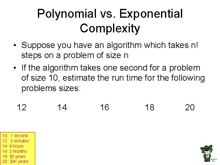
Polynomial vs. Exponential Complexity • Suppose you have an algorithm which takes n! steps on a problem of size n • If the algorithm takes one second for a problem of size 10, estimate the run time for the following problems sizes: 12 10: 1 second 12: 2 minutes 14: 6 hours 16: 2 months 18: 50 years 20: 20 K years 14 16 18 20

Ignoring constant factors • Express run time as O(f(n)) • Emphasize algorithms with slower growth rates • Fundamental idea in the study of algorithms • Basis of Tarjan/Hopcroft Turing Award

Why ignore constant factors? • Constant factors are arbitrary – Depend on the implementation – Depend on the details of the model • Determining the constant factors is tedious and provides little insight

Why emphasize growth rates? • The algorithm with the lower growth rate will be faster for all but a finite number of cases • Performance is most important for larger problem size • As memory prices continue to fall, bigger problem sizes become feasible • Improving growth rate often requires new techniques

Formalizing growth rates • T(n) is O(f(n)) [T : Z+ R+] – If n is sufficiently large, T(n) is bounded by a constant multiple of f(n) – Exist c, n 0, such that for n > n 0, T(n) < c f(n) • T(n) is O(f(n)) will be written as: T(n) = O(f(n)) – Be careful with this notation

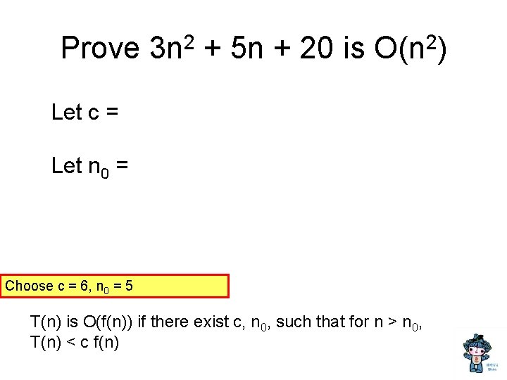
Prove 3 n 2 + 5 n + 20 is O(n 2) Let c = Let n 0 = Choose c = 6, n 0 = 5 T(n) is O(f(n)) if there exist c, n 0, such that for n > n 0, T(n) < c f(n)

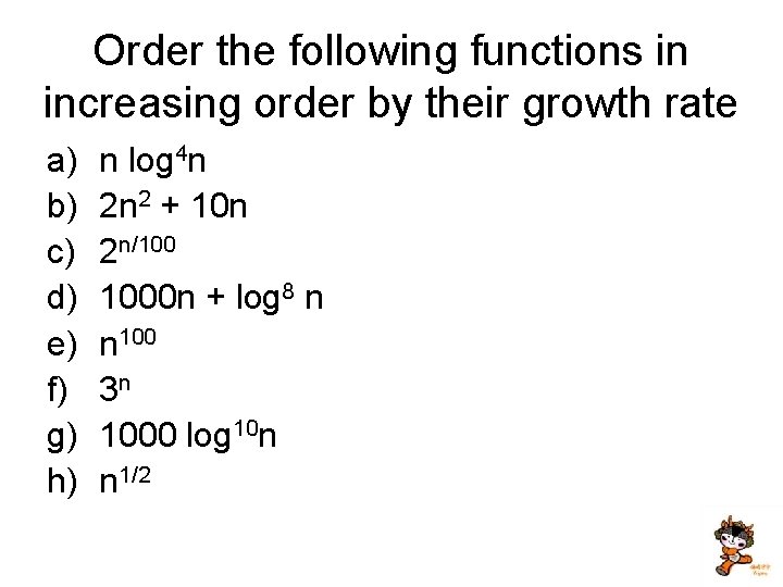
Order the following functions in increasing order by their growth rate a) b) c) d) e) f) g) h) n log 4 n 2 n 2 + 10 n 2 n/100 1000 n + log 8 n n 100 3 n 1000 log 10 n n 1/2

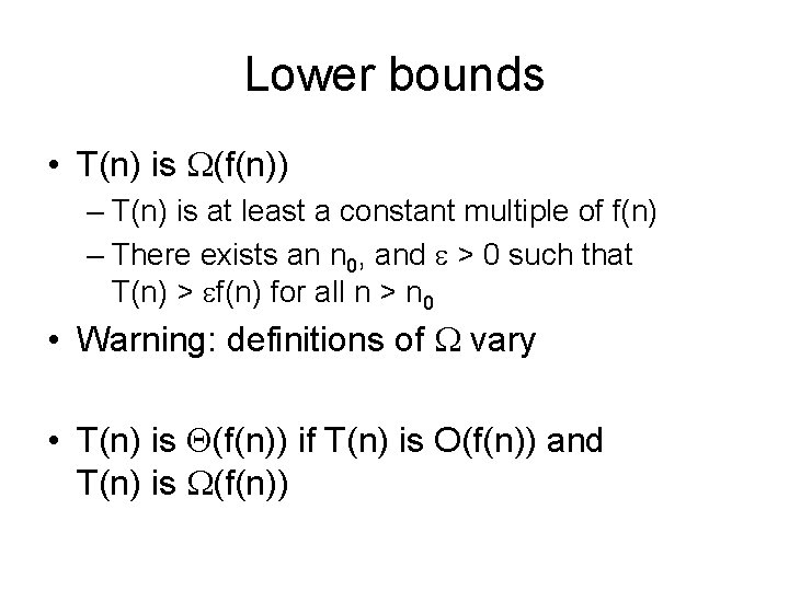
Lower bounds • T(n) is W(f(n)) – T(n) is at least a constant multiple of f(n) – There exists an n 0, and e > 0 such that T(n) > ef(n) for all n > n 0 • Warning: definitions of W vary • T(n) is Q(f(n)) if T(n) is O(f(n)) and T(n) is W(f(n))

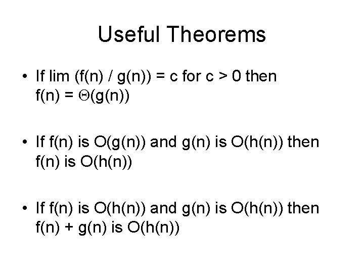
Useful Theorems • If lim (f(n) / g(n)) = c for c > 0 then f(n) = Q(g(n)) • If f(n) is O(g(n)) and g(n) is O(h(n)) then f(n) is O(h(n)) • If f(n) is O(h(n)) and g(n) is O(h(n)) then f(n) + g(n) is O(h(n))

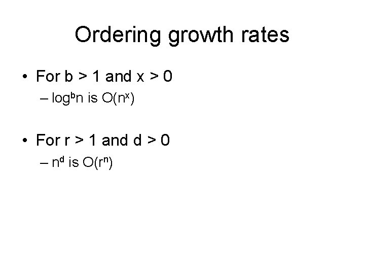
Ordering growth rates • For b > 1 and x > 0 – logbn is O(nx) • For r > 1 and d > 0 – nd is O(rn)

Formalizing growth rates • T(n) is O(f(n)) [T : Z+ R+] – If n is sufficiently large, T(n) is bounded by a constant multiple of f(n) – Exist c, n 0, such that for n > n 0, T(n) < c f(n) • T(n) is O(f(n)) will be written as: T(n) = O(f(n)) – Be careful with this notation

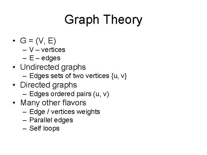
Graph Theory • G = (V, E) – V – vertices – E – edges • Undirected graphs – Edges sets of two vertices {u, v} • Directed graphs – Edges ordered pairs (u, v) • Many other flavors – Edge / vertices weights – Parallel edges – Self loops

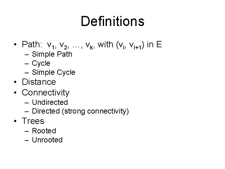
Definitions • Path: v 1, v 2, …, vk, with (vi, vi+1) in E – Simple Path – Cycle – Simple Cycle • Distance • Connectivity – Undirected – Directed (strong connectivity) • Trees – Rooted – Unrooted

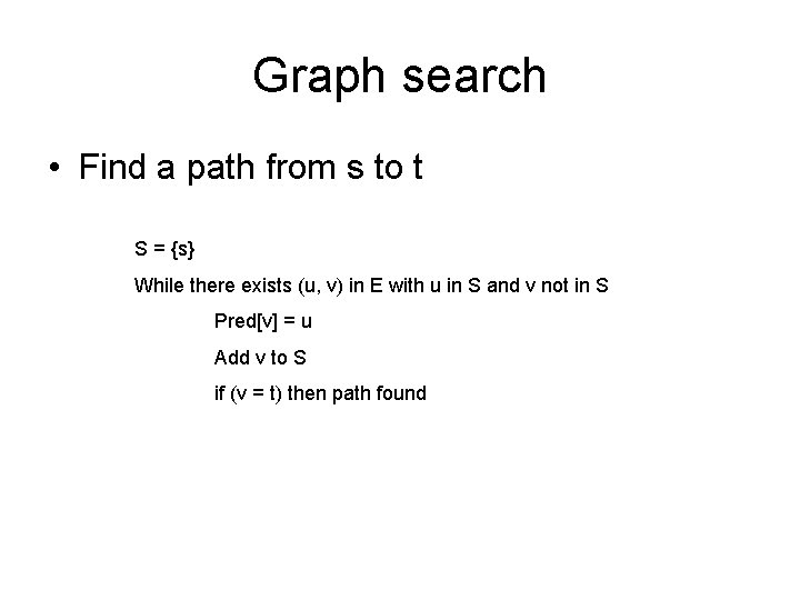
Graph search • Find a path from s to t S = {s} While there exists (u, v) in E with u in S and v not in S Pred[v] = u Add v to S if (v = t) then path found

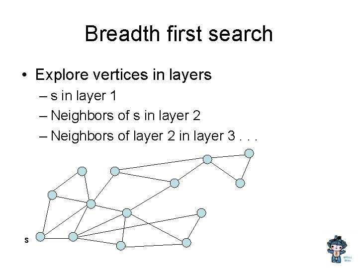
Breadth first search • Explore vertices in layers – s in layer 1 – Neighbors of s in layer 2 – Neighbors of layer 2 in layer 3. . . s

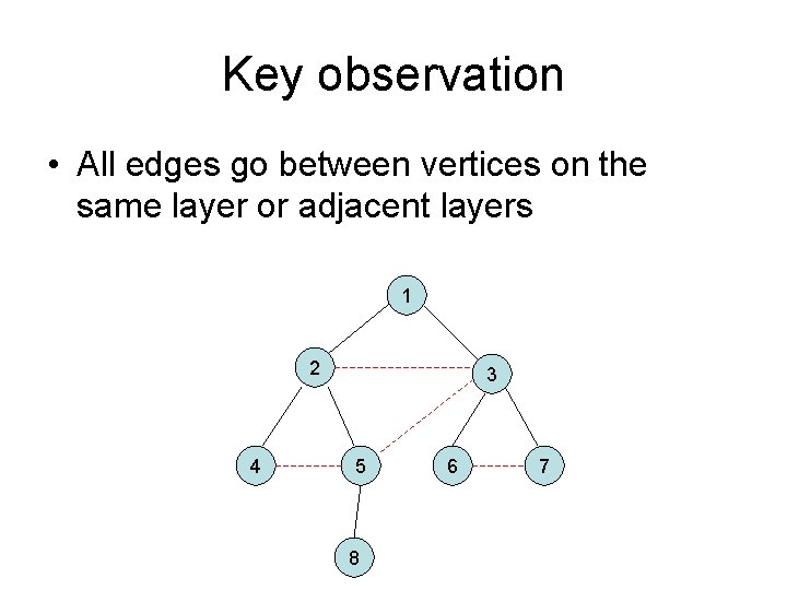
Key observation • All edges go between vertices on the same layer or adjacent layers 1 2 4 3 5 8 6 7

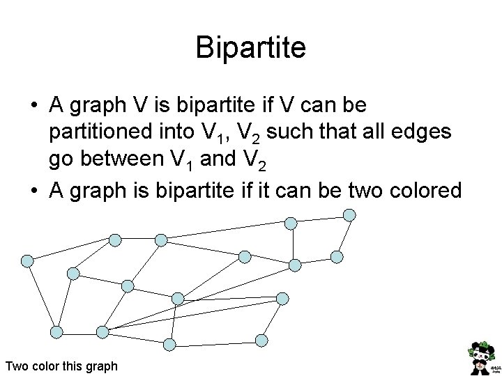
Bipartite • A graph V is bipartite if V can be partitioned into V 1, V 2 such that all edges go between V 1 and V 2 • A graph is bipartite if it can be two colored Two color this graph

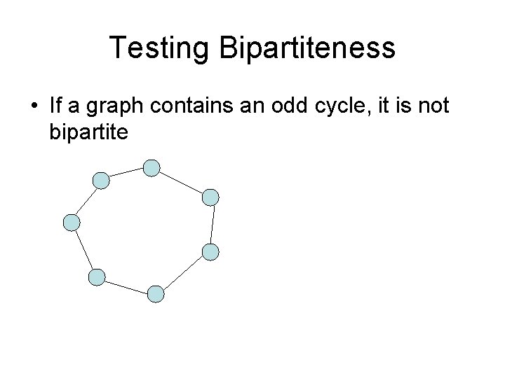
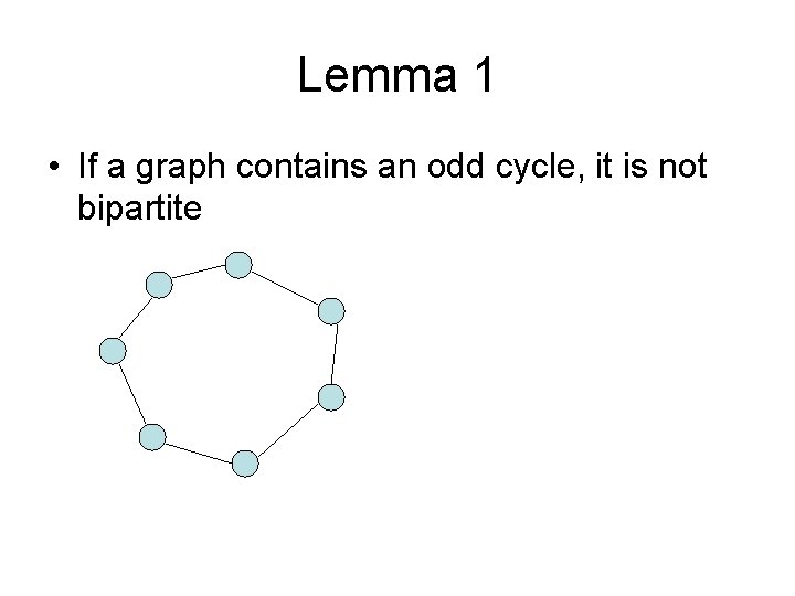
Testing Bipartiteness • If a graph contains an odd cycle, it is not bipartite

Algorithm • Run BFS • Color odd layers red, even layers blue • If no edges between the same layer, the graph is bipartite • If edge between two vertices of the same layer, then there is an odd cycle, and the graph is not bipartite

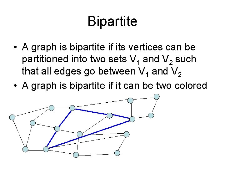
Bipartite • A graph is bipartite if its vertices can be partitioned into two sets V 1 and V 2 such that all edges go between V 1 and V 2 • A graph is bipartite if it can be two colored

Theorem: A graph is bipartite if and only if it has no odd cycles

Lemma 1 • If a graph contains an odd cycle, it is not bipartite

Lemma 2 • If a BFS tree has an intra-level edge, then the graph has an odd length cycle Intra-level edge: both end points are in the same level

Lemma 3 • If a graph has no odd length cycles, then it is bipartite

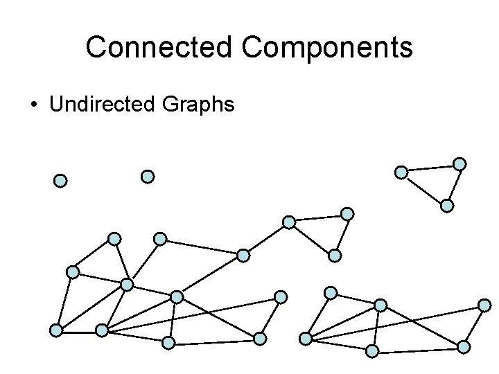
Connected Components • Undirected Graphs

Computing Connected Components in O(n+m) time • A search algorithm from a vertex v can find all vertices in v’s component • While there is an unvisited vertex v, search from v to find a new component

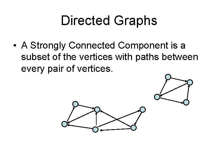
Directed Graphs • A Strongly Connected Component is a subset of the vertices with paths between every pair of vertices.

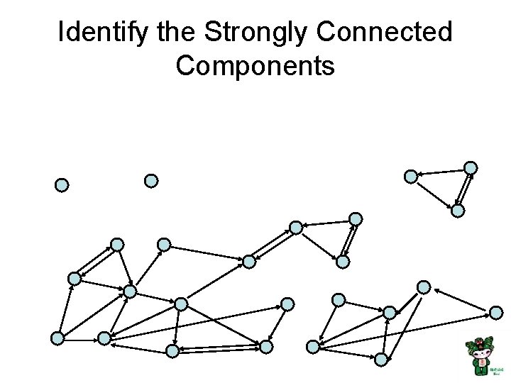
Identify the Strongly Connected Components

Strongly connected components can be found in O(n+m) time • But it’s tricky! • Simpler problem: given a vertex v, compute the vertices in v’s scc in O(n+m) time

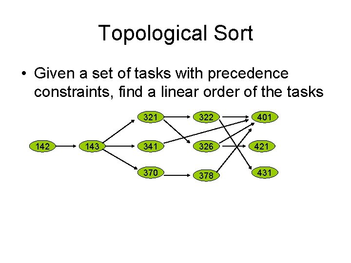
Topological Sort • Given a set of tasks with precedence constraints, find a linear order of the tasks 142 143 321 322 341 326 370 378 401 421 431

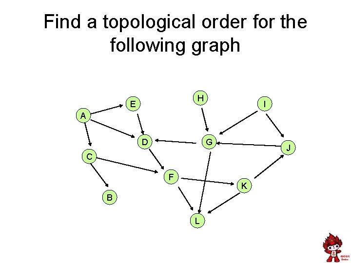
Find a topological order for the following graph H E I A D G J C F K B L

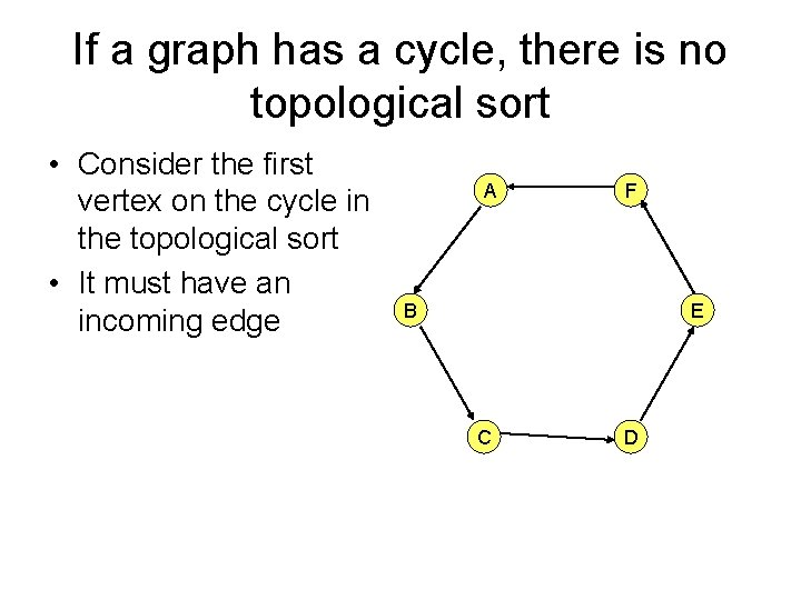
If a graph has a cycle, there is no topological sort • Consider the first vertex on the cycle in the topological sort • It must have an incoming edge A F B E C D

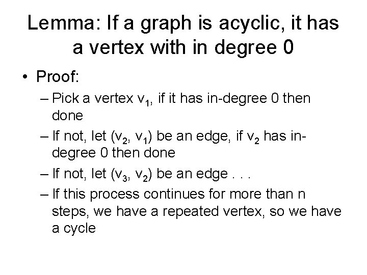
Lemma: If a graph is acyclic, it has a vertex with in degree 0 • Proof: – Pick a vertex v 1, if it has in-degree 0 then done – If not, let (v 2, v 1) be an edge, if v 2 has indegree 0 then done – If not, let (v 3, v 2) be an edge. . . – If this process continues for more than n steps, we have a repeated vertex, so we have a cycle

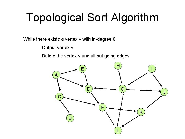
Topological Sort Algorithm While there exists a vertex v with in-degree 0 Output vertex v Delete the vertex v and all out going edges H E I A D G J C F K B L

Details for O(n+m) implementation • Maintain a list of vertices of in-degree 0 • Each vertex keeps track of its in-degree • Update in-degrees and list when edges are removed • m edge removals at O(1) cost each