Support Vector Machine ITCS 6190 Cloud Computing in

Support Vector Machine ITCS 6190 - Cloud Computing in Data Analysis

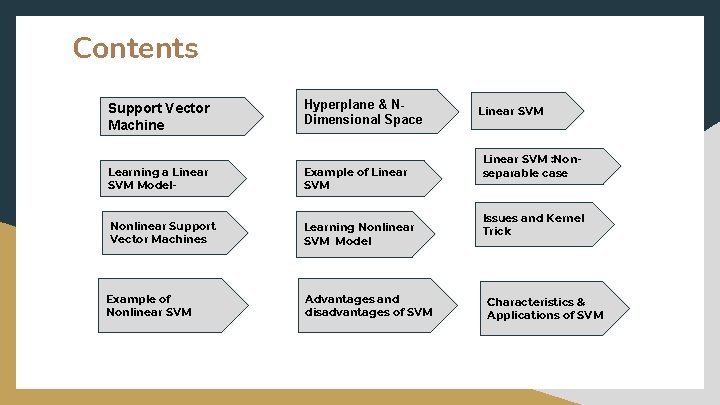
Contents Support Vector Machine Hyperplane & NDimensional Space Learning a Linear SVM Model- Example of Linear SVM Nonlinear Support Vector Machines Learning Nonlinear SVM Model Example of Nonlinear SVM Advantages and disadvantages of SVM Linear SVM : Nonseparable case Issues and Kernel Trick Characteristics & Applications of SVM

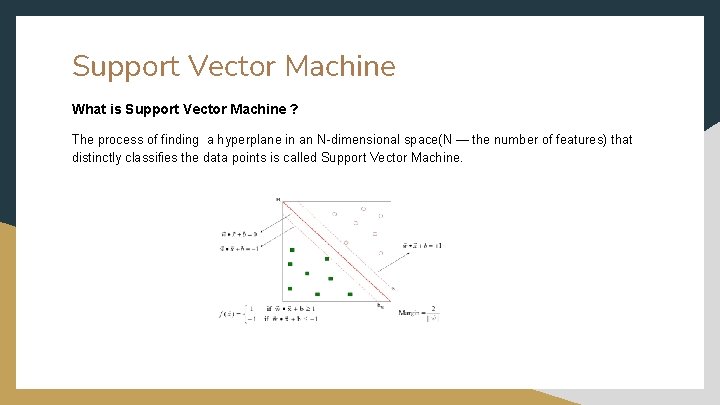
Support Vector Machine What is Support Vector Machine ? The process of finding a hyperplane in an N-dimensional space(N — the number of features) that distinctly classifies the data points is called Support Vector Machine.

Characteristics of SVM ● Since the learning problem is formulated as a convex optimization problem, efficient algorithms are available to find the global minima of the objective function (many of the other methods use greedy approaches and find locally optimal solutions) ● Overfitting is addressed by maximizing the margin of the decision boundary, but the user still needs to provide the type of kernel function and cost function ● Difficult to handle missing values ● Robust to noise ● High computational complexity for building the model

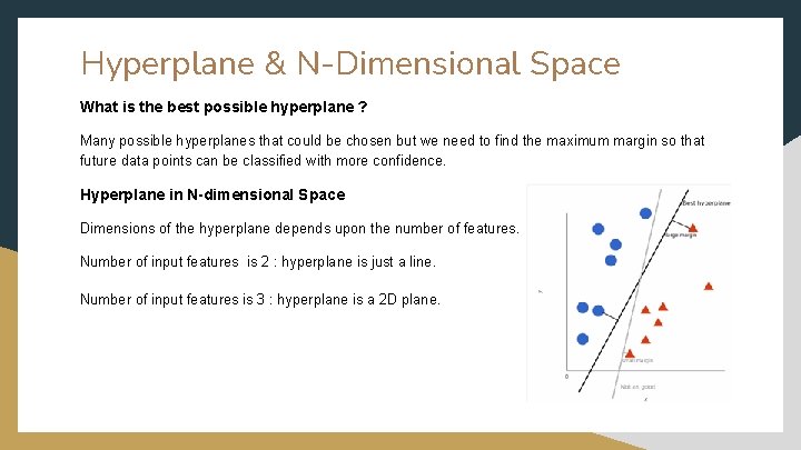
Hyperplane & N-Dimensional Space What is the best possible hyperplane ? Many possible hyperplanes that could be chosen but we need to find the maximum margin so that future data points can be classified with more confidence. Hyperplane in N-dimensional Space Dimensions of the hyperplane depends upon the number of features. Number of input features is 2 : hyperplane is just a line. Number of input features is 3 : hyperplane is a 2 D plane.

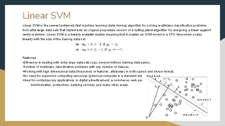
Linear SVM is the newest extremely fast machine learning (data mining) algorithm for solving multiclassification problems from ultra large data sets that implements an original proprietary version of a cutting plane algorithm for designing a linear support vector machine. Linear SVM is a linearly scalable routine meaning that it creates an SVM model in a CPU time which scales linearly with the size of the training data set. Features • Efficiency in dealing with extra large data sets (say, several millions training data pairs), • Solution of multiclassification problems with any number of classes, • Working with high dimensional data (thousands of features, attributes) in both sparse and dense format, • No need for expensive computing resources (personal computer is a standard platform), • Ideal for contemporary applications in digital advertisement, e-commerce, web page categorization, text classification, bioinformatics, proteomics, banking services and many other areas.

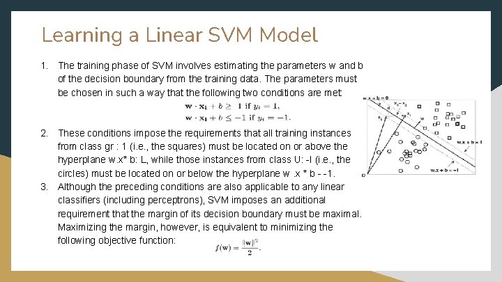
Learning a Linear SVM Model 1. The training phase of SVM involves estimating the parameters w and b of the decision boundary from the training data. The parameters must be chosen in such a way that the following two conditions are met: 2. These conditions impose the requirements that all training instances from class gr : 1 (i. e. , the squares) must be located on or above the hyperplane w. x* b: L, while those instances from class U: -I (i. e. , the circles) must be located on or below the hyperplane w. x * b - -1. 3. Although the preceding conditions are also applicable to any linear classifiers (including perceptrons), SVM imposes an additional requirement that the margin of its decision boundary must be maximal. Maximizing the margin, however, is equivalent to minimizing the following objective function:

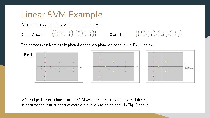
Linear SVM Example Assume our dataset has two classes as follows: Class A data = Class B = The dataset can be visually plotted on the x-y plane as seen in the Fig. 1 below: Fig 1. Fig 2. ❖Our objective is to find a linear SVM which can classify the given dataset. ❖Assume that our support vectors are chosen to be as seen in Fig. 2 above; Fig 3

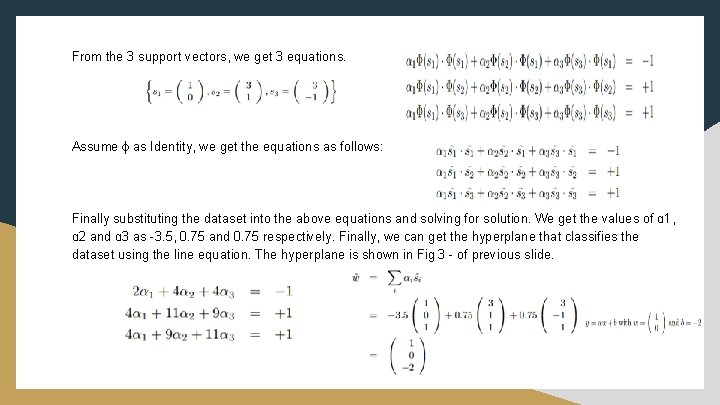
From the 3 support vectors, we get 3 equations. Assume ɸ as Identity, we get the equations as follows: Finally substituting the dataset into the above equations and solving for solution. We get the values of ɑ 1, ɑ 2 and ɑ 3 as -3. 5, 0. 75 and 0. 75 respectively. Finally, we can get the hyperplane that classifies the dataset using the line equation. The hyperplane is shown in Fig 3 - of previous slide.

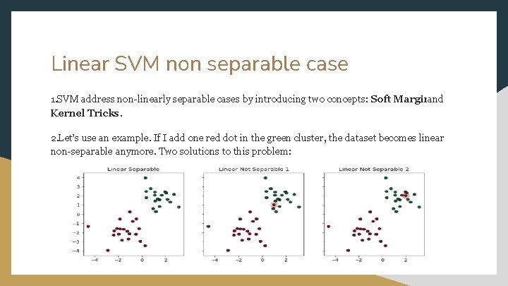
Linear SVM non separable case 1. SVM address non-linearly separable cases by introducing two concepts: Soft Marginand Kernel Tricks. 2. Let’s use an example. If I add one red dot in the green cluster, the dataset becomes linear non-separable anymore. Two solutions to this problem:

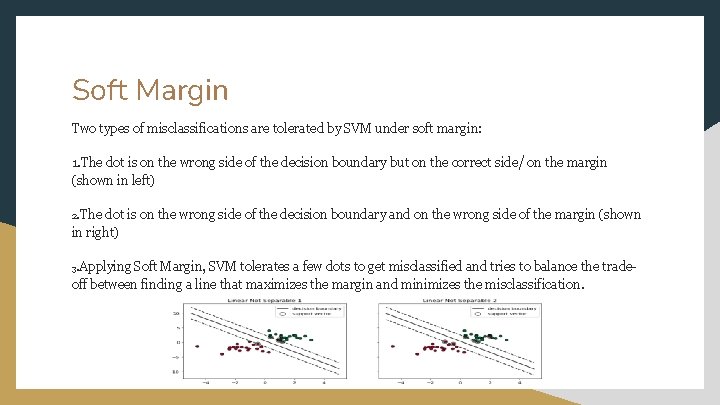
Soft Margin Two types of misclassifications are tolerated by SVM under soft margin: 1. The dot is on the wrong side of the decision boundary but on the correct side/ on the margin (shown in left) 2. The dot is on the wrong side of the decision boundary and on the wrong side of the margin (shown in right) 3. Applying Soft Margin, SVM tolerates a few dots to get misclassified and tries to balance the tradeoff between finding a line that maximizes the margin and minimizes the misclassification.

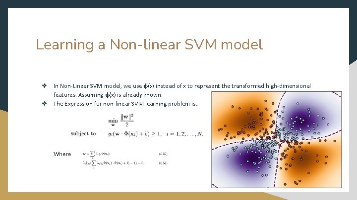
Non Linear SVM ● ● ● Non Linear SVM are used to project data that is not linearly separable into a higher dimensional space. A non linear transformation is needed to map the date from its original feature space into new space where the decision boundary becomes linear. Different methodologies are used to find a linear decision boundary in the transformed space after performing the above transformation. Parameters can be found in the transformed space. One potential problem with this approach is that it may suffer from the curse of dimensionality problem often associated with high-dimensional data. Non linear SVM can avoid this problem by using kernel trick.

Learning a Non-linear SVM model ❖ In Non-Linear SVM model, we use φ(x) instead of x to represent the transformed high-dimensional features. Assuming φ(x) is already known. φ ❖ The Expression for non-linear SVM learning problem is: Where

Kernel Trick ● Kernel trick method is used by SVM to perform a non-linear classification. ● Kernel trick is used to learn a linear classifier to classify a non-linear dataset. ● It transforms the linearly inseparable data into a linearly separable one by projecting it into a higher dimension. ● A kernel function is applied on each data instance to map the original nonlinear data points into some higher dimensional space in which they become linearly separable.

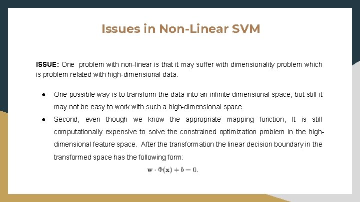
Issues in Non-Linear SVM ISSUE: One problem with non-linear is that it may suffer with dimensionality problem which is problem related with high-dimensional data. ● One possible way is to transform the data into an infinite dimensional space, but still it may not be easy to work with such a high-dimensional space. ● Second, even though we know the appropriate mapping function, It is still computationally expensive to solve the constrained optimization problem in the highdimensional feature space. After the transformation the linear decision boundary in the transformed space has the following form:

Advantages and Disadvantages of SVM Advantages ● ● SVM works relatively well when there is clear margin of separation between classes. SVM is more efficient in high dimensional spaces. Disadvantages ● ● SVM algorithm is not suitable for large data sets. SVM does not perform very well when the data set has more noise i. e target classes are overlapping.

Real World Applications of SVM ● ● ● Face detection - SVM classify parts of the image as a face and non face and create a square boundary around the face Classification of images - use of SVM’s provide better search accuracy for image classification. It provides better accuracy in terms in comparison to the traditional based query-based searching techniques. Handwriting recognition - We use SVMs to recognize handwritten characters used widely.