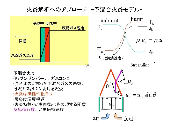
Stream lines outer flame Inner flame air premixed

Stream lines outer flame Inner flame air premixed flow air fuel typical burner flame temperature Fundaments of Combustion & Flame distance along streamline pre-heated layer flame propagation reaction layer diffusion layer fuel burnt gas unburnt gas premixed flame (inner flame) oxygen reaction range diffusion flame (outer flame)

Weak points of G-equation modeling 1. 2. A pure convection equation tends unstable in numerical solution without diffusion term. An initial profile is conserved in time evolution， even if inappropriate. ？？ a. Use upwind scheme or add numerical diffusion. b. Reset the profile adjusted to physical or mathematical meaning; ex. distance function. 　　　（level-set method）

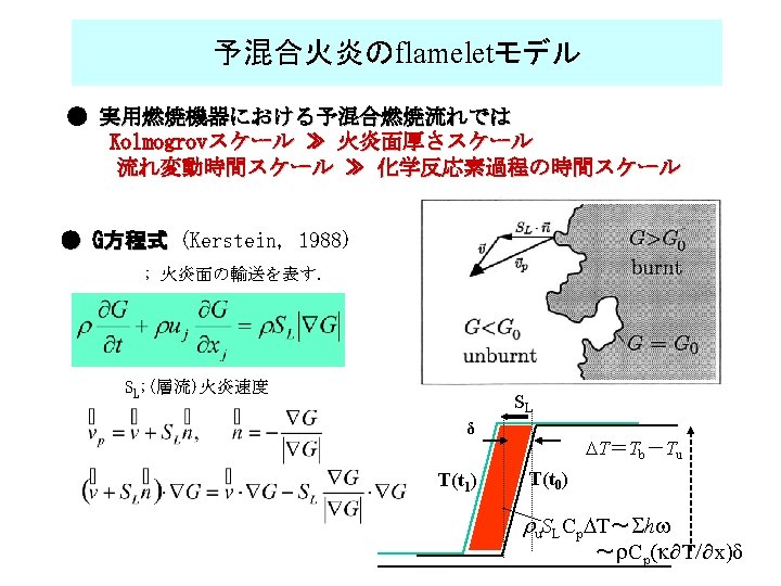
Analysis of local profile near the flame surface 1 D plane flame ru d ru. Su • Considering a finite thickness d Unburnt (G<0) – Add a diffusion term explicitly, – Give a spatial profile of S 　 by Taylor’s expansion around G= G 0 ，・・・ Burnt (0<G) x G 未燃 ， G=G 0 d 既燃 X

Burger’s eq. hyperbolic tangent profile ,

Analysis of profile in the flame • Dependency on variation of r (analogy of ru = const. ) • Density weighted flame speed if and

Analysis of profile in the flame (cont. ’d) In laminar plane flame ( ); n Dependency on Variation of G ( )

１ D example 1 D Flame propagation by 　 new G-eq. old G-eq. new 25 steps old 100 steps old+diff. 100 steps X [mm] Fig. 1 Time marching solution of new eq. from linear initial profile for CH 4: O 2: N 2=1: 2: 3 premixed flame. X [mm] Fig. 2 Time marching solutions of new and old eqs. from the same linear initial profile.

0. 0002[s] ２ D example • Curvature effect on local flame speed rounds the flame shape. 0. 0102[s] • Fluid dynamic flame instability by converging/diverging stream lines. 0. 0302[s] Burnt gas flow out 0. 0702[s] 0. 1102[s] Fig. 4 G-profile and steam lines at 0. 1802[s]

Analysis of solution around a spherical flame 3 D formulation • Cylindrical (r-q) coordinate 　(n: dimension) 　　　　　 on flame surface Su : expand r iｆ u=0, G=G 0, : shrink (extinct)

Analysis of solution with a streching flow • Flame in a stretching flow L: Markstain No. (～ 1) (Calvin 1985) burnt • Flame speed dependency Constant flame speed d x u unburnt

Modeling for Partially Premixed Flame Methane-air lifted non-premixed jet flame Muniz and Mungal, Combustion and flame 111, 1997 fuel tube inner diameter D=4. 8 [mm] SL 0 max of methane-air flame=0. 37[m] (for ex. Re=4900, avaraged Lift-off height is about 30 D=150 [mm]) (www. efluids. com) 60 D Fuel CH 4 (99% Vol. ) AIR Coflow Inlet diameter D=4. 8　(mm) Velocity (Fuel ) Ujet=15. 0 [m/s] Velocity(Co-flow ) Uco=0. 74 [m/s] Reynolds No. 4900 20 D air D Fuel Domain ( X, R, θ)= (60 D, 2π) No. of Grid cells(X, R, θ)=(200, 82, 32)

Classification of the flame position Classification of Chen et al. (2000) FLAME C FLAME A Air Fuel Blow-out criterion Edge flame extinction Triple flame propagation Frame-front propagation

2 scalar flamelet model of partially premixed flame Flamelet equation Diffusion flame, Mixing of Fuel Mixture fraction equation Premixed flame propagation Flamelet. G-equation Lifted diffusion flame RANS: Muller et al(1994), Herrmann et al. (2000) LES: Duchamp et al (2001), LES: Hirohata et al(2001) Schematic Figure of Triple flame

Mass fraction model using 2 scalar flamelet. Air x=xst Burnt gas: Diffusion flame zone Fuel Un-burnt gas: Mixing zone Partial Premixed flame front G=G 0 The G-equation is used to distinguish between the unburnt and burnt regions, the iso-surface of G is used to express flame surface. Unburnt mixing zone (G=0) flame surface(G=0. 5) Diffusion flame zone (G=1)

Quenching effect of turbulent burning velocity L: Markstain No. (～ 1) Burnt gas with quenching model Burnt gas without quenching model fq=1 Flame tips can not quench where the strong shear exists Lift-off height and flame shape cannot be predicted without quenching model.

Premixed flame with the mixture rate gradient • Flame speed dependency on defined position based on the flamelet approach G=0. 25 G=0. 75 18

Premixed flame with the mixture rate gradient – Fuel ratio (ξ) gradient normal to flame surface (G) – Flame speed SL is basically depend on ξ Is flame speed same as simple plane flame? iso-surface of G=0. 5 19

Premixed flame with the mixture rate gradient • mixture rate gradient normal to flame face ⇒ gradient of flame speed ⇒ thinner flame Flame speed gradient on the flame surface : turbulent flame thickness : turbulent flame speed gradient 20

Level-set to phase field in flame • Distance function (scale in space) G G=G(x) unburnt x 　 d burnt X • Progress variable (scale in time) plane laminar flame corrugated or wrinkling turbulent flame d d x : distance from flame surface x’: observed distance in averaged flame x (~x’): real distance along streamlimes gas flow d’ ＞ d ：observed thickness (if s’/d’ ～ s/d)

Level-set to phase field in flame Steady propagating flame solution: =0 Level-set form if S 1→ 0 　(S 1/G=const) thin flame assumption If steady solution exists, =const Phase field form (F ~ quadratic)

Level-set to phase field in flame Inage’s Hyperbolic Tangent Approximation (Inage et. al. 1989) h: progress variable Example CHEMKIN　（GRI-Mech 3. 0） CH 4 - O 2 (φ=1) ＋ N 2 50%　300 K temperature Assumed solution for laminar plane flame: CHEMKIN 1400+1100 tanh{(x-x 0)/d} x ［mm］

PH for non-equilibrium flame interface Allen-Cahn equation(Allen & Cahn 1979, Chen 1992) This formulation insure the second law of thermal mechanics, so that F(h) (=Free energy) decreases in time Model of steady liquid-solid phase interface (vf=0) 1 D plane surface: F（h） h Model of growing liquid-solid phase interface

PH for non-equilibrium flame interface Functional F(h) of Allen-Cahn eq. h Gibbs’ free energy progresses in CH 4/air flame q (K) 1 0 G (k. J/kg) Reaction slow F(h) Reaction fast Reaction slow Source term fitting to Inage’s model Gibbs’ free energy: G=H-TS for gas reaction in constant pressure Thermal equilibrium CAN’T be assumed in a flame with large temperature change.

Based on Phase Field Method (Fife 2000) Modified A-C eq. for temperature variation Estimated by numerical solution Inage’s model Mf(h) CHEMKIN solution of homogeneous condition CH 4 -O 2 (stoichimetric 600 K) Compare to Inage’s model h

PH for non-equilibrium flame interface Modified A-C eq. with internal heat sink (Fife 2000) h→S： Entropy H(=rc. T): Enthalpy is conserved F→G(S, T)：Gibbs’free energy e S Sb Su Local homogeneous Approx. Tb T ru Internal heat sink by convection holds a steady flame. Tu x Local equilibrium assumed in a steady flame (T locally balanced). ⇔ analogy to spinodal phase change

PH for non-equilibrium flame interface Modified A-C eq. for gas reaction with large temperature raise Estimation in flame: Tb: burnt gas temperature (under H=const. & rc. Tu ≪DTS) Reactions stop at burnt region： M(T) corresponds to the reaction speed which should increase as temperature raise：

PH for non-equilibrium flame interface Modified A-C eq. for gas reaction with large temperature raise Tb: burnt gas temperature (under H=const. & rc. Tu ≪DTS) Ex. CH 4/Air premixed flame TS[KJ] [D] [C 1] [C 2] [B] [A] by num. solution in homogeneous [B] 　　　is estimated [C 1] by num. solution in homogeneous [C 2] and [A] T[K] [D] Inage’s model

Conclusive remarks • Modified level-set function for premixed flamelet (G-eq) is derived to consider the flame thickness. • Inage’s flame model (progress variable) is considered by phase-field method based on Allen-Cahn eq. • Modified level-set function is consistent to phase-field method based on Allen-Cahn eq. , where the hyperbolic tangent profile is a