Statistical Leverage and Improved Matrix Algorithms Michael W

Statistical Leverage and Improved Matrix Algorithms Michael W. Mahoney Stanford University

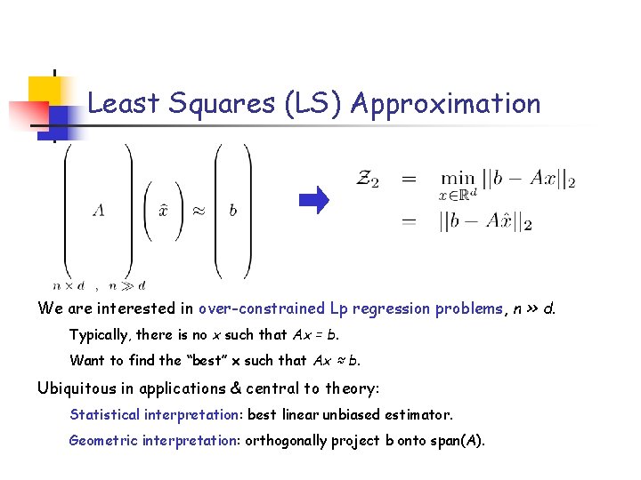
Least Squares (LS) Approximation We are interested in over-constrained Lp regression problems, n >> d. Typically, there is no x such that Ax = b. Want to find the “best” x such that Ax ≈ b. Ubiquitous in applications & central to theory: Statistical interpretation: best linear unbiased estimator. Geometric interpretation: orthogonally project b onto span(A).

Many applications of this! • Astronomy: Predicting the orbit of the asteroid Ceres (in 1801!). Gauss (1809) -- see also Legendre (1805) and Adrain (1808). First application of “least squares optimization” and runs in O(nd 2) time! • Bioinformatics: Dimension reduction for classification of gene expression microarray data. • Medicine: Inverse treatment planning and fast intensity-modulated radiation therapy. • Engineering: Finite elements methods for solving Poisson, etc. equation. • Control theory: Optimal design and control theory problems. • Economics: Restricted maximum-likelihood estimation in econometrics. • Image Analysis: Array signal and image processing. • Computer Science: Computer vision, document and information retrieval. • Internet Analysis: Filtering and de-noising of noisy internet data. • Data analysis: Fit parameters of a biological, chemical, economic, social, internet, etc. model to experimental data.

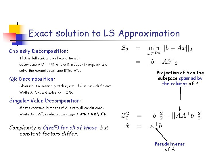
Exact solution to LS Approximation Cholesky Decomposition: If A is full rank and well-conditioned, decompose ATA = RTR, where R is upper triangular, and solve the normal equations: RTRx=ATb. QR Decomposition: Slower but numerically stable, esp. if A is rank-deficient. Projection of b on the subspace spanned by the columns of A Write A=QR, and solve Rx = QTb. Singular Value Decomposition: Most expensive, but best if A is very ill-conditioned. Write A=U VT, in which case: x. OPT = A+b = V -1 k. UTb. Complexity is O(nd 2) for all of these, but constant factors differ. Pseudoinverse of A

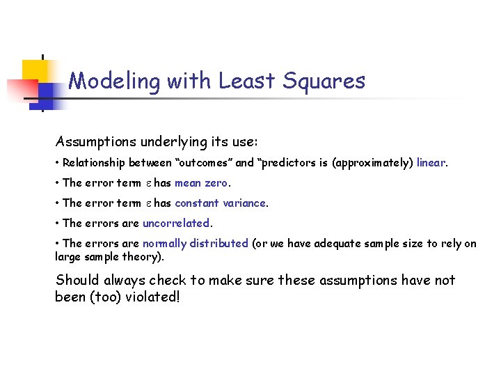
Modeling with Least Squares Assumptions underlying its use: • Relationship between “outcomes” and “predictors is (approximately) linear. • The error term has mean zero. • The error term has constant variance. • The errors are uncorrelated. • The errors are normally distributed (or we have adequate sample size to rely on large sample theory). Should always check to make sure these assumptions have not been (too) violated!

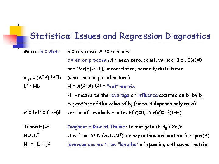
Statistical Issues and Regression Diagnostics Model: b = Ax+ b = response; A(i) = carriers; = error process s. t. : mean zero, const. varnce, (i. e. , E(e)=0 and Var(e)= 2 I), uncorrelated, normally distributed xopt = (ATA)-1 ATb (what we computed before) b’ = Hb H = A(ATA)-1 AT = “hat” matrix Hij - measures the leverage or influence exerted on b’i by bj, regardless of the value of bj (since H depends only on A) e’ = b-b’ = (I-H)b vector of residuals - note: E(e’)=0, Var(e’)= 2(I-H) Trace(H)=d Diagnostic Rule of Thumb: Investigate if Hii > 2 d/n H=UUT U is from SVD (A=U VT), or any orthogonal matrix for span(A) Hii = |U(i)|22 leverage scores = row “lengths” of spanning orthogonal matrix

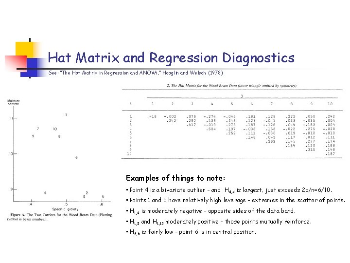
Hat Matrix and Regression Diagnostics See: “The Hat Matrix in Regression and ANOVA, ” Hoaglin and Welsch (1978) Examples of things to note: • Point 4 is a bivariate outlier - and H 4, 4 is largest, just exceeds 2 p/n=6/10. • Points 1 and 3 have relatively high leverage - extremes in the scatter of points. • H 1, 4 is moderately negative - opposite sides of the data band. • H 1, 8 and H 1, 10 moderately positive - those points mutually reinforce. • H 6, 6 is fairly low - point 6 is in central position.

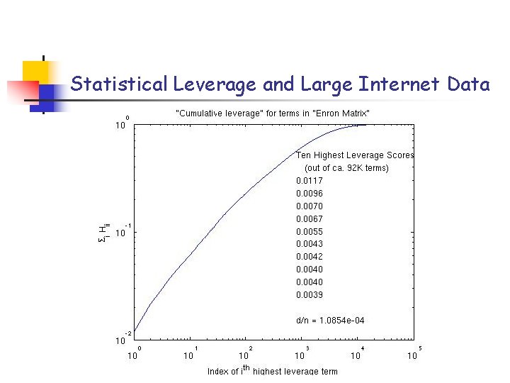
Statistical Leverage and Large Internet Data

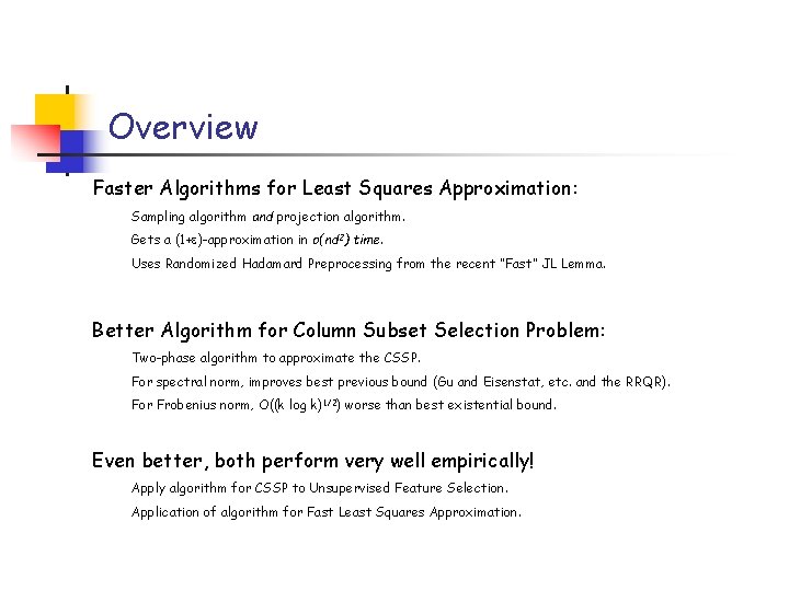
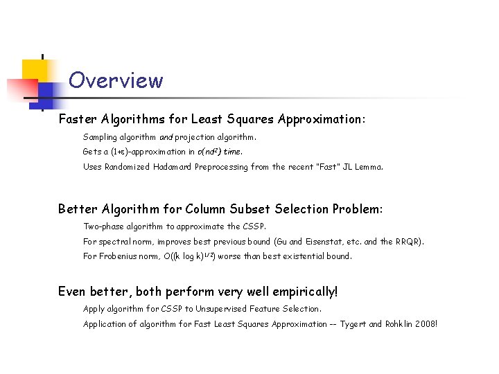
Overview Faster Algorithms for Least Squares Approximation: Sampling algorithm and projection algorithm. Gets a (1+ )-approximation in o(nd 2) time. Uses Randomized Hadamard Preprocessing from the recent “Fast” JL Lemma. Better Algorithm for Column Subset Selection Problem: Two-phase algorithm to approximate the CSSP. For spectral norm, improves best previous bound (Gu and Eisenstat, etc. and the RRQR). For Frobenius norm, O((k log k)1/2) worse than best existential bound. Even better, both perform very well empirically! Apply algorithm for CSSP to Unsupervised Feature Selection. Application of algorithm for Fast Least Squares Approximation.

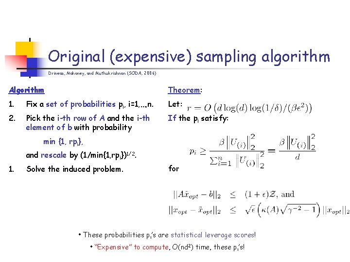
Original (expensive) sampling algorithm Drineas, Mahoney, and Muthukrishnan (SODA, 2006) Algorithm Theorem: 1. Fix a set of probabilities pi, i=1, …, n. Let: 2. Pick the i-th row of A and the i-th element of b with probability If the pi satisfy: min {1, rpi}, and rescale by (1/min{1, rpi})1/2. 1. Solve the induced problem. for some (0, 1], then w. p. ≥ 1 - , • These probabilities pi’s are statistical leverage scores! • “Expensive” to compute, O(nd 2) time, these pi’s!

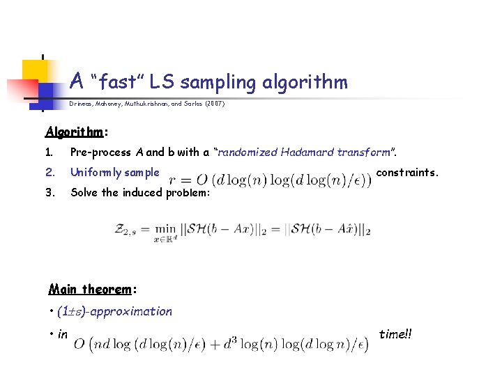
A “fast” LS sampling algorithm Drineas, Mahoney, Muthukrishnan, and Sarlos (2007) Algorithm: 1. Pre-process A and b with a “randomized Hadamard transform”. 2. Uniformly sample 3. Solve the induced problem: constraints. Main theorem: • (1 )-approximation • in time!!

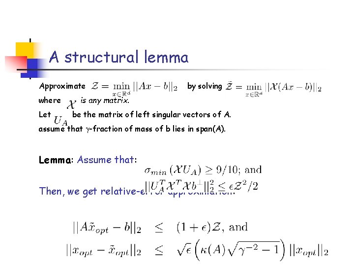
A structural lemma Approximate where Let by solving is any matrix. be the matrix of left singular vectors of A. assume that -fraction of mass of b lies in span(A). Lemma: Assume that: Then, we get relative-error approximation:

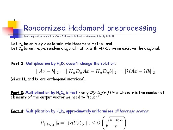
Randomized Hadamard preprocessing Facts implicit or explicit in: Ailon & Chazelle (2006), or Ailon and Liberty (2008). Let Hn be an n-by-n deterministic Hadamard matrix, and Let Dn be an n-by-n random diagonal matrix with +1/-1 chosen u. a. r. on the diagonal. Fact 1: Multiplication by Hn. Dn doesn’t change the solution: (since Hn and Dn are orthogonal matrices). Fact 2: Multiplication by Hn. Dn is fast - only O(n log(r)) time, where r is the number of elements of the output vector we need to “touch”. Fact 3: Multiplication by Hn. Dn approximately uniformizes all leverage scores:

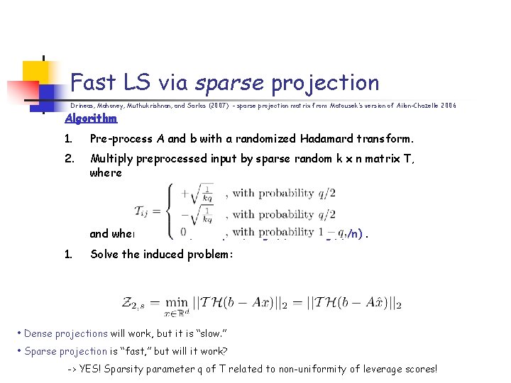
Fast LS via sparse projection Drineas, Mahoney, Muthukrishnan, and Sarlos (2007) - sparse projection matrix from Matousek’s version of Ailon-Chazelle 2006 Algorithm 1. Pre-process A and b with a randomized Hadamard transform. 2. Multiply preprocessed input by sparse random k x n matrix T, where and where k=O(d/ ) and q=O(d log 2(n)/n+d 2 log(n)/n). 1. Solve the induced problem: • Dense projections will work, but it is “slow. ” • Sparse projection is “fast, ” but will it work? -> YES! Sparsity parameter q of T related to non-uniformity of leverage scores!

Overview Faster Algorithms for Least Squares Approximation: Sampling algorithm and projection algorithm. Gets a (1+ )-approximation in o(nd 2) time. Uses Randomized Hadamard Preprocessing from the recent “Fast” JL Lemma. Better Algorithm for Column Subset Selection Problem: Two-phase algorithm to approximate the CSSP. For spectral norm, improves best previous bound (Gu and Eisenstat, etc. and the RRQR). For Frobenius norm, O((k log k)1/2) worse than best existential bound. Even better, both perform very well empirically! Apply algorithm for CSSP to Unsupervised Feature Selection. Application of algorithm for Fast Least Squares Approximation.

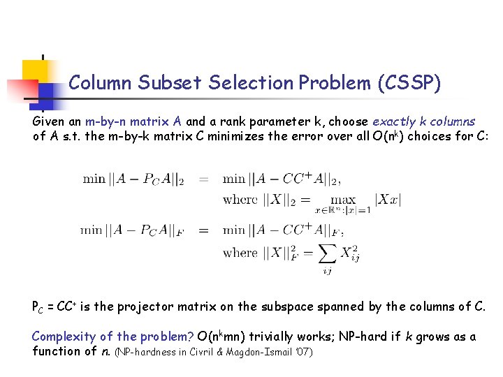
Column Subset Selection Problem (CSSP) Given an m-by-n matrix A and a rank parameter k, choose exactly k columns of A s. t. the m-by-k matrix C minimizes the error over all O(nk) choices for C: PC = CC+ is the projector matrix on the subspace spanned by the columns of C. Complexity of the problem? O(nkmn) trivially works; NP-hard if k grows as a function of n. (NP-hardness in Civril & Magdon-Ismail ’ 07)

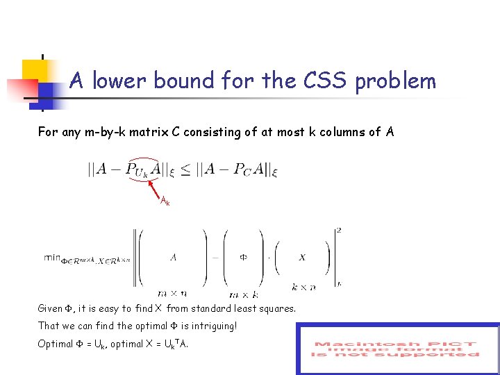
A lower bound for the CSS problem For any m-by-k matrix C consisting of at most k columns of A Ak Given , it is easy to find X from standard least squares. That we can find the optimal is intriguing! Optimal = Uk, optimal X = Uk. TA.

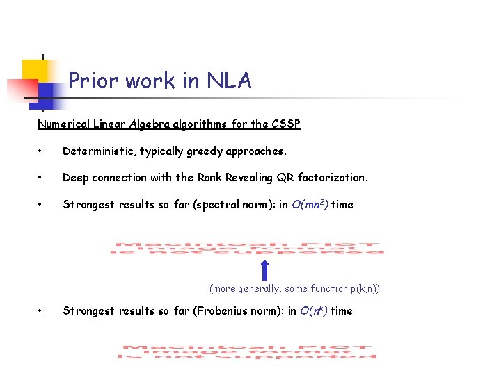
Prior work in NLA Numerical Linear Algebra algorithms for the CSSP • Deterministic, typically greedy approaches. • Deep connection with the Rank Revealing QR factorization. • Strongest results so far (spectral norm): in O(mn 2) time (more generally, some function p(k, n)) • Strongest results so far (Frobenius norm): in O(nk) time

Working on p(k, n): 1965 – today

Theoretical computer science contributions Theoretical Computer Science algorithms for the CSSP 1. Randomized approaches, with some failure probability. 2. More than k columns are picked, e. g. , O(poly(k)) columns chosen. 3. Very strong bounds for the Frobenius norm in low polynomial time. 4. Not many spectral norm bounds.

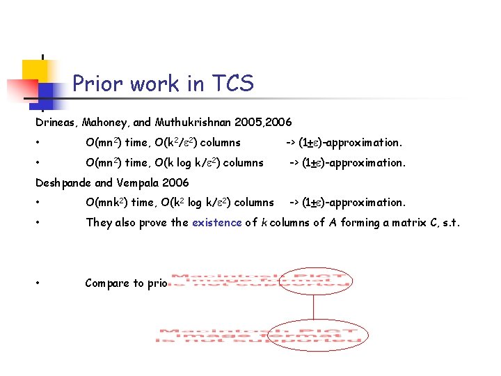
Prior work in TCS Drineas, Mahoney, and Muthukrishnan 2005, 2006 • O(mn 2) time, O(k 2/ 2) columns -> (1± )-approximation. • O(mn 2) time, O(k log k/ 2) columns -> (1± )-approximation. Deshpande and Vempala 2006 • O(mnk 2) time, O(k 2 log k/ 2) columns • They also prove the existence of k columns of A forming a matrix C, s. t. • Compare to prior best existence result: -> (1± )-approximation.

The strongest Frobenius norm bound Drineas, Mahoney, and Muthukrishnan (2006) Theorem: Given an m-by-n matrix A, there exists an O(mn 2) algorithm that picks at most O( k log k / 2 ) columns of A such that with probability at least 1 -10 -20 Algorithm: Use subspace sampling probabilities to sample O(k log k / 2 ) columns.

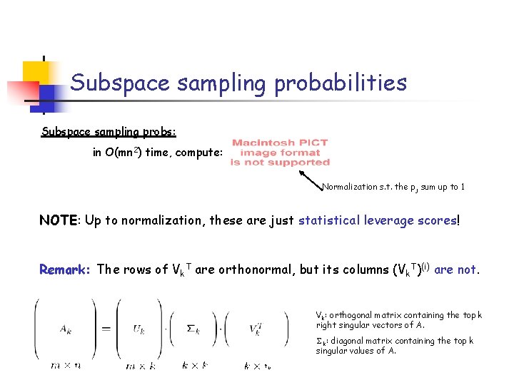
Subspace sampling probabilities Subspace sampling probs: in O(mn 2) time, compute: Normalization s. t. the pj sum up to 1 NOTE: Up to normalization, these are just statistical leverage scores! Remark: The rows of Vk. T are orthonormal, but its columns (Vk. T)(i) are not. Vk: orthogonal matrix containing the top k right singular vectors of A. k: diagonal matrix containing the top k singular values of A.

Prior work bridging NLA/TCS Woolfe, Liberty, Rohklin, and Tygert 2007 (also Martinsson, Rohklin, and Tygert 2006) • O(mn log k) time, k columns • Same spectral norm bounds as prior work • Application of the Fast Johnson-Lindenstrauss transform of Ailon-Chazelle • Nice empirical evaluation. How to improve bounds for CSSP? • Not obvious that bounds improve if allow NLA to choose more columns. • Not obvious how to get around TCS need to over-sample to O(k log(k)) to preserve rank.

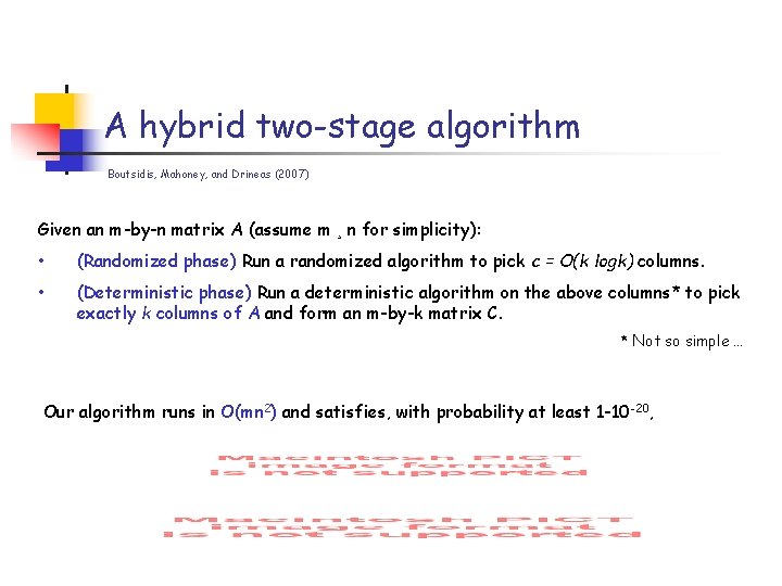
A hybrid two-stage algorithm Boutsidis, Mahoney, and Drineas (2007) Given an m-by-n matrix A (assume m ¸ n for simplicity): • (Randomized phase) Run a randomized algorithm to pick c = O(k logk) columns. • (Deterministic phase) Run a deterministic algorithm on the above columns* to pick exactly k columns of A and form an m-by-k matrix C. * Not so simple … Our algorithm runs in O(mn 2) and satisfies, with probability at least 1 -10 -20,

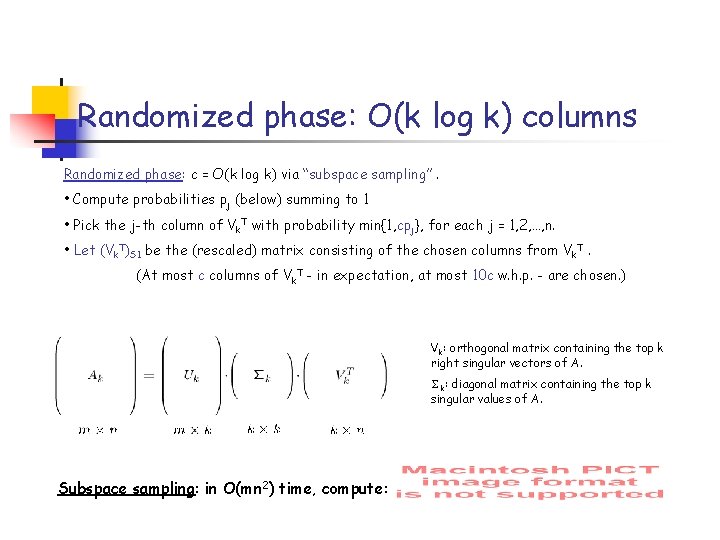
Randomized phase: O(k log k) columns Randomized phase: c = O(k log k) via “subspace sampling”. • Compute probabilities pj (below) summing to 1 • Pick the j-th column of Vk. T with probability min{1, cpj}, for each j = 1, 2, …, n. • Let (Vk. T)S 1 be the (rescaled) matrix consisting of the chosen columns from Vk. T. (At most c columns of Vk. T - in expectation, at most 10 c w. h. p. - are chosen. ) Vk: orthogonal matrix containing the top k right singular vectors of A. k: diagonal matrix containing the top k singular values of A. Subspace sampling: in O(mn 2) time, compute:

Deterministic phase: exactly k columns Deterministic phase • Let S 1 be the set of indices of the columns selected by the randomized phase. • Let (Vk. T)S 1 denote the set of columns of Vk. T with indices in S 1, (Technicality: the columns of (Vk. T)S 1 must be rescaled. ) • Run a deterministic NLA algorithm on (Vk. T)S 1 to select exactly k columns. (Any algorithm with p(k, n) = k 1/2(n-k)1/2 will do. ) • Let S 2 be the set of indices of the selected columns. (The cardinality of S 2 is exactly k. ) • Return AS 2 as the final ourput. (That is, return the columns of A corresponding to indices in S 2. )

Analysis of the two-stage algorithm Lemma 1: k(Vk. TS 1 D 1) ≥ 1/2. (By matrix perturbation lemma, subspace sampling, and since c=O(k log(k). ) Lemma 2: ||A-PCA|| ≤ ||A-Ak|| + k-1(Vk. TS 1 D 1 S 2)|| -k. V -k. TS 1 D 1||. Lemma 3: k-1(Vk. TS 1 D 1 S 2) ≤ 2(k(c-k+1))1/2. (Combine Lemma 1 with the NLA bound from the deterministic phase on the c - not n - columns of Vk. TS 1 D 1. ) Lemma 4&5: || -k. V -k. TS 1 D 1|| ≈ ||A-Ak|| , for =2, F.

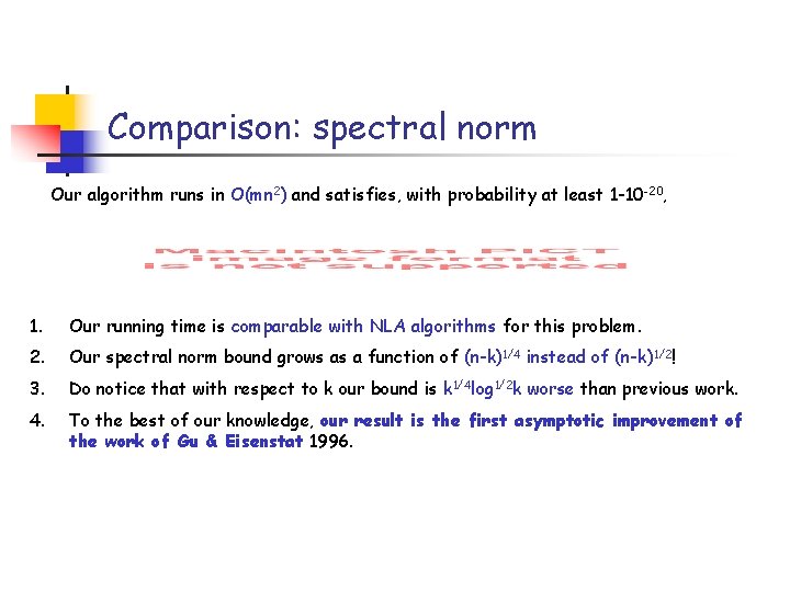
Comparison: spectral norm Our algorithm runs in O(mn 2) and satisfies, with probability at least 1 -10 -20, 1. Our running time is comparable with NLA algorithms for this problem. 2. Our spectral norm bound grows as a function of (n-k)1/4 instead of (n-k)1/2! 3. Do notice that with respect to k our bound is k 1/4 log 1/2 k worse than previous work. 4. To the best of our knowledge, our result is the first asymptotic improvement of the work of Gu & Eisenstat 1996.

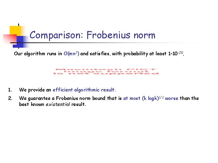
Comparison: Frobenius norm Our algorithm runs in O(mn 2) and satisfies, with probability at least 1 -10 -20, 1. We provide an efficient algorithmic result. 2. We guarantee a Frobenius norm bound that is at most (k logk)1/2 worse than the best known existential result.

Overview Faster Algorithms for Least Squares Approximation: Sampling algorithm and projection algorithm. Gets a (1+ )-approximation in o(nd 2) time. Uses Randomized Hadamard Preprocessing from the recent “Fast” JL Lemma. Better Algorithm for Column Subset Selection Problem: Two-phase algorithm to approximate the CSSP. For spectral norm, improves best previous bound (Gu and Eisenstat, etc. and the RRQR). For Frobenius norm, O((k log k)1/2) worse than best existential bound. Even better, both perform very well empirically! Apply algorithm for CSSP to Unsupervised Feature Selection. Application of algorithm for Fast Least Squares Approximation -- Tygert and Rohklin 2008!

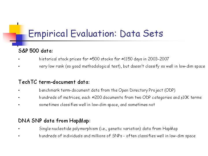
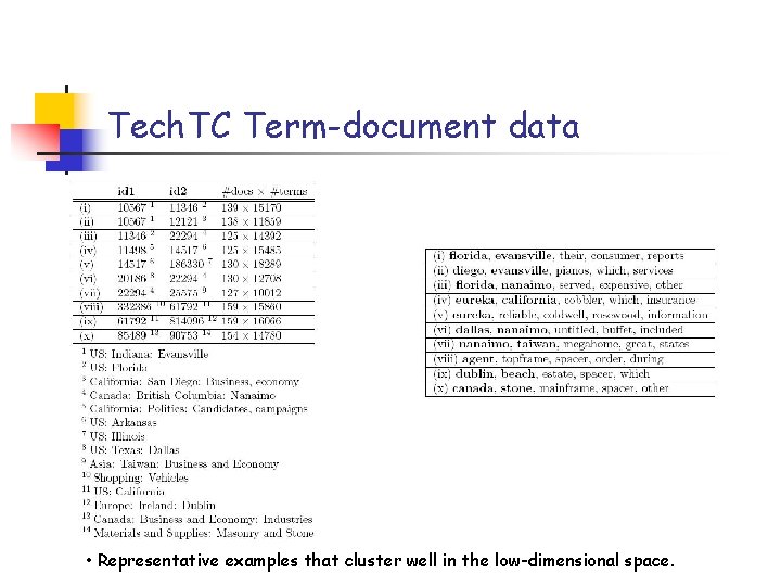
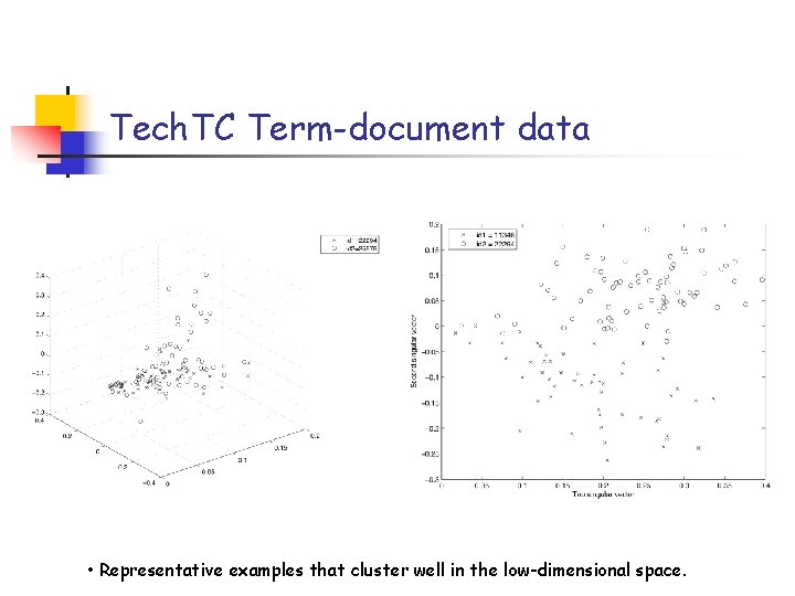
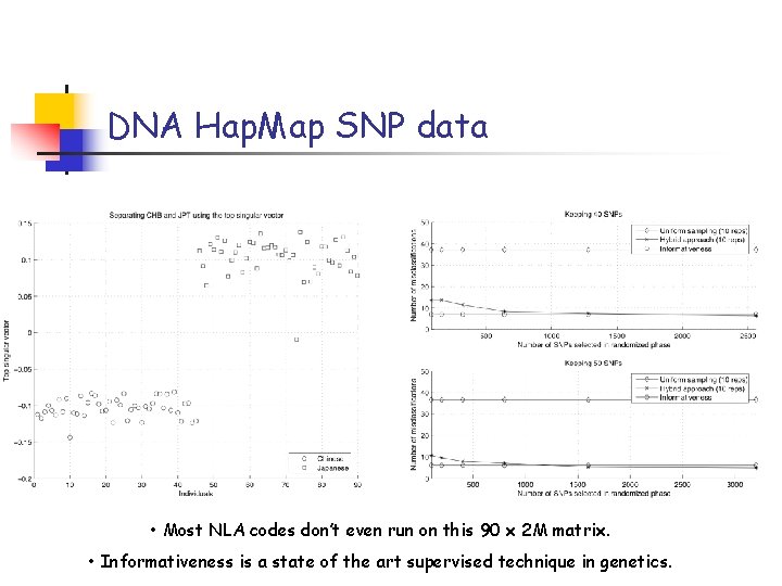
Empirical Evaluation: Data Sets S&P 500 data: • historical stock prices for ≈500 stocks for ≈1150 days in 2003 -2007 • very low rank (so good methodological test), but doesn’t classify so well in low-dim space Tech. TC term-document data: • benchmark term-document data from the Open Directory Project (ODP) • hundreds of matrices, each ≈200 documents from two ODP categories and ≥ 10 K terms • sometimes classifies well in low-dim space, and sometimes not DNA SNP data from Hap. Map: • Single nucleotide polymorphism (i. e. , genetic variation) data from Hap. Map • hundreds of individuals and millions of SNPs - often classifies well in low-dim space

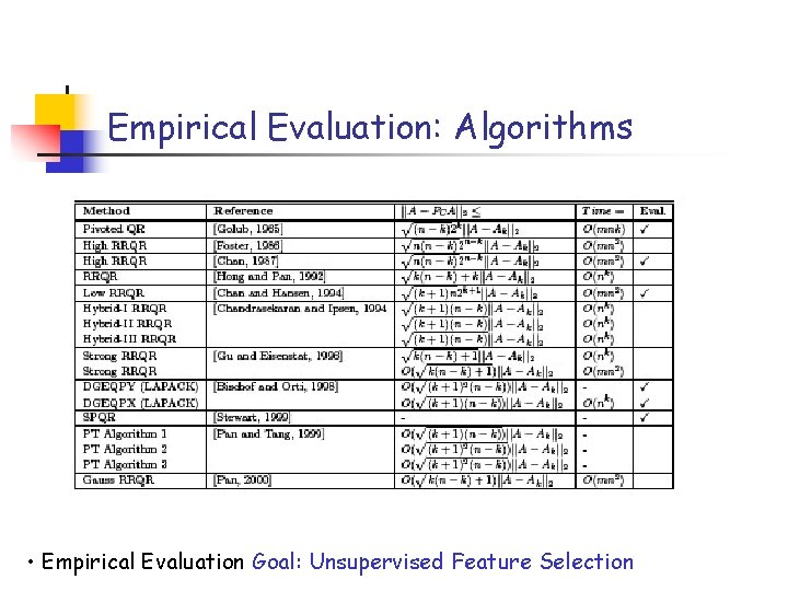
Empirical Evaluation: Algorithms • Empirical Evaluation Goal: Unsupervised Feature Selection

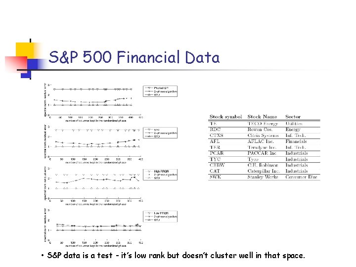
S&P 500 Financial Data • S&P data is a test - it’s low rank but doesn’t cluster well in that space.

Tech. TC Term-document data • Representative examples that cluster well in the low-dimensional space.

Tech. TC Term-document data • Representative examples that cluster well in the low-dimensional space.

Tech. TC Term-document data

DNA Hap. Map SNP data • Most NLA codes don’t even run on this 90 x 2 M matrix. • Informativeness is a state of the art supervised technique in genetics.

DNA Hap. Map SNP data

Conclusion Faster Algorithms for Least Squares Approximation: Sampling algorithm and projection algorithm. Gets a (1+ )-approximation in o(nd 2) time. Uses Randomized Hadamard Preprocessing from the recent “Fast” JL Lemma. Better Algorithm for Column Subset Selection Problem: Two-phase algorithm to approximate the CSSP. For spectral norm, improves best previous bound (Gu and Eisenstat, etc. and the RRQR). For Frobenius norm, O((k log k)1/2) worse than best existential bound. Even better, both perform very well empirically! Apply algorithm for CSSP to Unsupervised Feature Selection. Application of algorithm for Fast Least Squares Approximation.