Stacks queues and DP ESC 101 Fundamentals of

Stacks, queues and DP ESC 101: Fundamentals of Computing Nisheeth 1

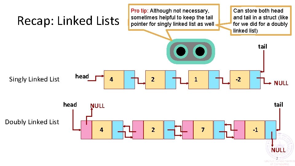
Recap: Linked Lists Pro tip: Although not necessary, sometimes helpful to keep the tail pointer for singly linked list as well Can store both head and tail in a struct (like for we did for a doubly linked list) tail Singly Linked List head Doubly Linked List 4 2 1 -2 NULL tail NULL 4 2 7 -1 NULL 2

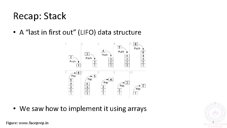
Recap: Stack • A “last in first out” (LIFO) data structure • We saw how to implement it using arrays Figure: www. faceprep. in 3

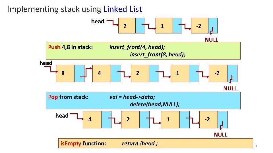
Implementing stack using Linked List head Push 4, 8 in stack: 2 1 -2 insert_front(4, head); insert_front(8, head); NULL head 8 4 2 1 -2 NULL Pop from stack: head 4 val = head->data; delete(head, NULL); 2 1 -2 NULL is. Empty function: return !head ; 4

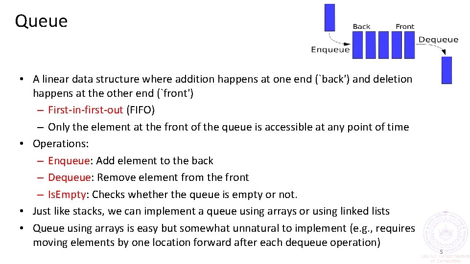
Queue • A linear data structure where addition happens at one end (`back') and deletion happens at the other end (`front') – First-in-first-out (FIFO) – Only the element at the front of the queue is accessible at any point of time • Operations: – Enqueue: Add element to the back – Dequeue: Remove element from the front – Is. Empty: Checks whether the queue is empty or not. • Just like stacks, we can implement a queue using arrays or using linked lists • Queue using arrays is easy but somewhat unnatural to implement (e. g. , requires moving elements by one location forward after each dequeue operation) 5

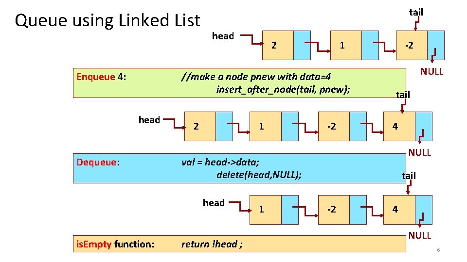
Queue using Linked List Enqueue 4: tail head 2 1 //make a node pnew with data=4 insert_after_node(tail, pnew); head Dequeue: 2 1 NULL tail 4 NULL val = head->data; delete(head, NULL); head is. Empty function: -2 -2 return !head ; 1 tail -2 4 NULL 6

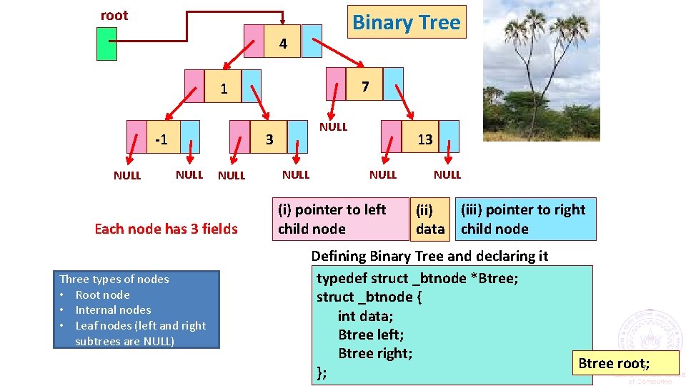
root Binary Tree 4 7 1 3 -1 NULL Each node has 3 fields Three types of nodes • Root node • Internal nodes • Leaf nodes (left and right subtrees are NULL) NULL 13 NULL (i) pointer to left child node NULL (ii) data (iii) pointer to right child node Defining Binary Tree and declaring it typedef struct _btnode *Btree; struct _btnode { int data; Btree left; Btree right; }; Btree root; 7

Dynamic Programming 8

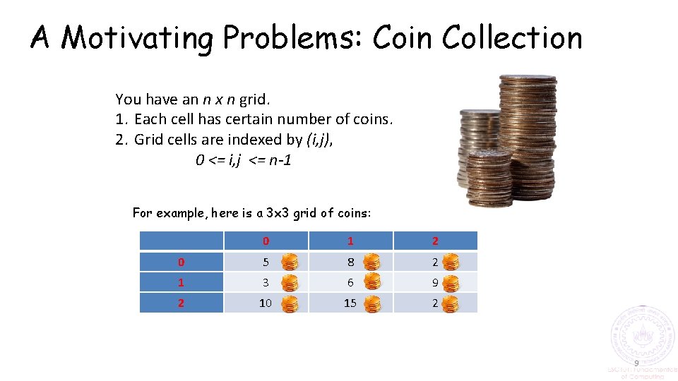
A Motivating Problems: Coin Collection You have an n x n grid. 1. Each cell has certain number of coins. 2. Grid cells are indexed by (i, j), 0 <= i, j <= n-1 For example, here is a 3 x 3 grid of coins: 0 1 2 0 5 8 2 1 3 6 9 2 10 15 2 9

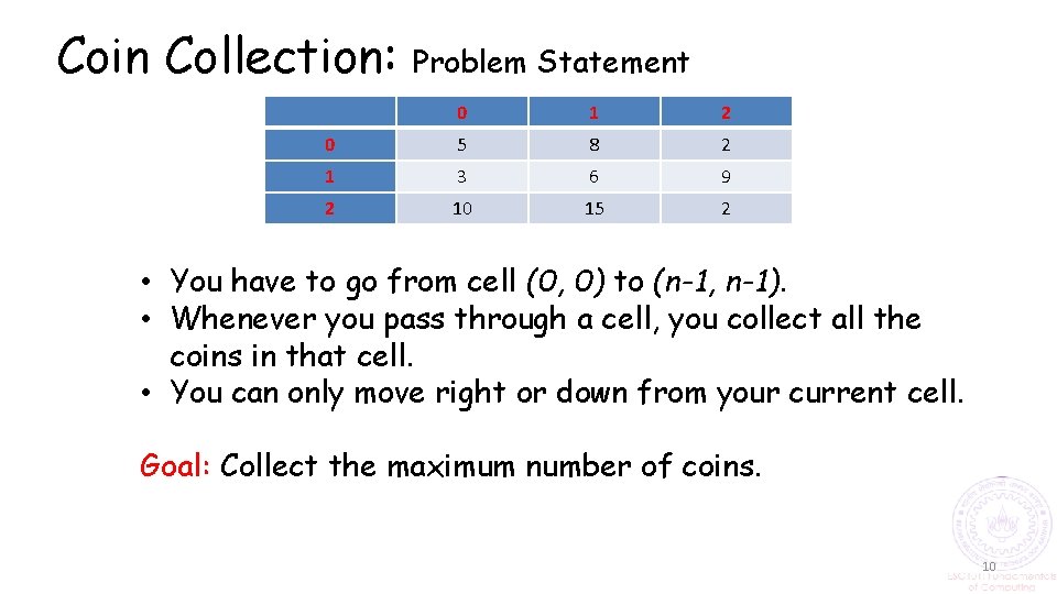
Coin Collection: Problem Statement 0 1 2 0 5 8 2 1 3 6 9 2 10 15 2 • You have to go from cell (0, 0) to (n-1, n-1). • Whenever you pass through a cell, you collect all the coins in that cell. • You can only move right or down from your current cell. Goal: Collect the maximum number of coins. 10

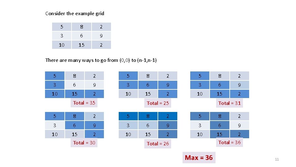
Consider the example grid 5 8 2 3 6 9 10 15 2 There are many ways to go from (0, 0) to (n-1, n-1) 5 8 2 3 6 9 10 15 2 Total = 35 Total = 25 Total = 31 5 8 2 3 6 9 10 15 2 Total = 30 10 15 2 Total = 36 Total = 26 Max = 36 11

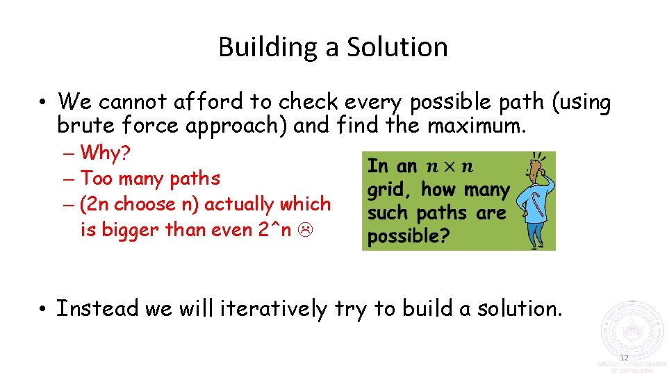
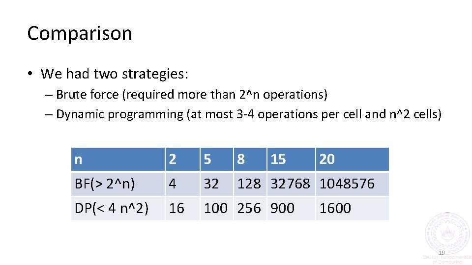
Building a Solution • We cannot afford to check every possible path (using brute force approach) and find the maximum. – Why? – Too many paths – (2 n choose n) actually which is bigger than even 2^n • Instead we will iteratively try to build a solution. 12

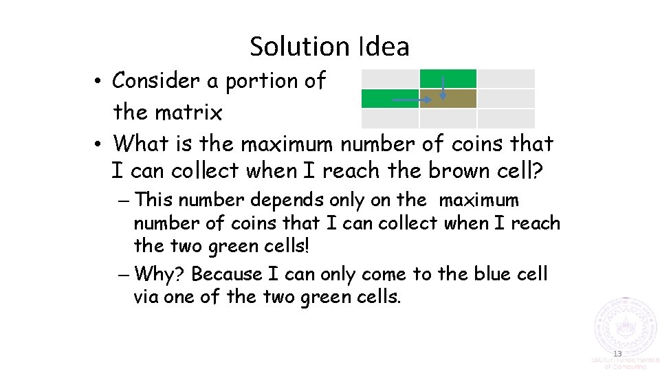
Solution Idea • Consider a portion of the matrix • What is the maximum number of coins that I can collect when I reach the brown cell? – This number depends only on the maximum number of coins that I can collect when I reach the two green cells! – Why? Because I can only come to the blue cell via one of the two green cells. 13

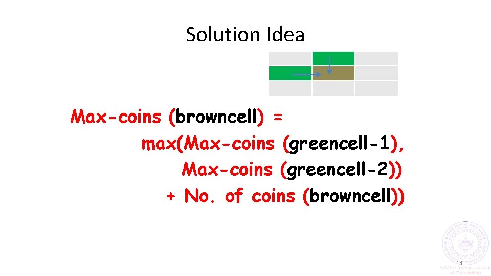
Solution Idea Max-coins (browncell) = max(Max-coins (greencell-1), Max-coins (greencell-2)) + No. of coins (browncell)) 14

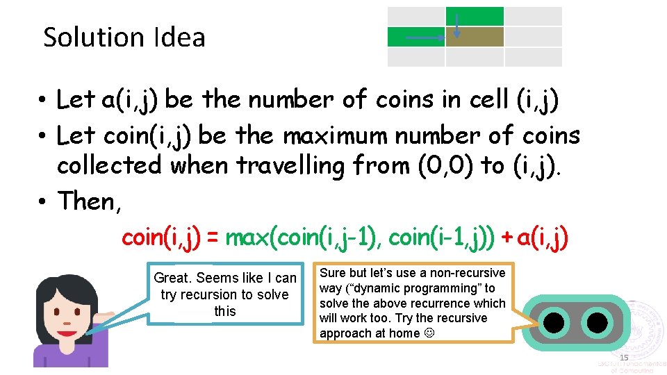
Solution Idea • Let a(i, j) be the number of coins in cell (i, j) • Let coin(i, j) be the maximum number of coins collected when travelling from (0, 0) to (i, j). • Then, coin(i, j) = max(coin(i, j-1), coin(i-1, j)) + a(i, j) Great. Seems like I can try recursion to solve this Sure but let’s use a non-recursive way (“dynamic programming” to solve the above recurrence which will work too. Try the recursive approach at home 15

A Non-recursive Implementation • Use an additional two dimensional array, whose (i, j)-th cell will store the maximum number of coins collected when travelling from (0, 0) to (i, j). • Fill this array one row at a time, from left to right. • When the array is completely filled, return the (n-1, n 1)-th element. 16

Implementation: Boundary Cases • To fill a cell of this array, we need to know the information of the cell above and to the left of the cell. • What about elements in the top most row and left most column? – Cell in top row: no cell above – Cell in leftmost column: no cell on left • Before starting with the other elements, we will fill these first. 17

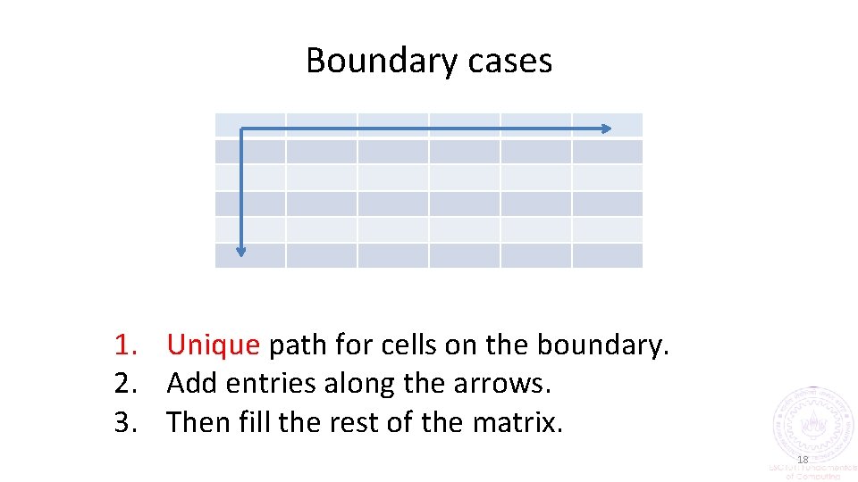
Boundary cases 1. Unique path for cells on the boundary. 2. Add entries along the arrows. 3. Then fill the rest of the matrix. 18

Comparison • We had two strategies: – Brute force (required more than 2^n operations) – Dynamic programming (at most 3 -4 operations per cell and n^2 cells) n 2 5 8 15 20 BF(> 2^n) 4 32 128 32768 1048576 DP(< 4 n^2) 16 100 256 900 1600 19

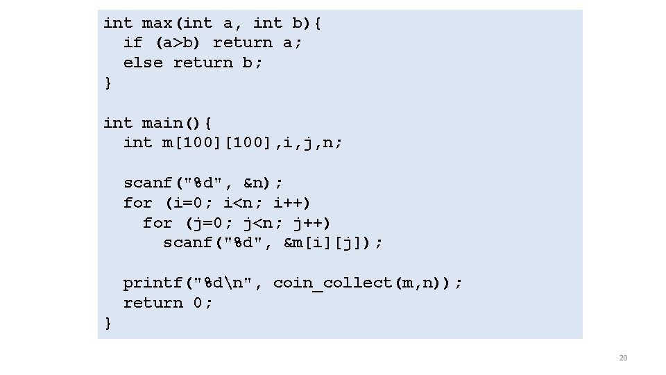
int max(int a, int b){ if (a>b) return a; else return b; } int main(){ int m[100], i, j, n; scanf("%d", &n); for (i=0; i<n; i++) for (j=0; j<n; j++) scanf("%d", &m[i][j]); printf("%dn", coin_collect(m, n)); return 0; } 20

int coin_collect(int a[][100], int n){ int i, j, coins[100]; coins[0][0] = a[0][0]; //initial cell for (i=1; i<n; i++) //first row coins[0][i] = coins[0][i-1] + a[0][i]; for (i=1; i<n; i++) //first column coins[i][0] = coins[i-1][0] + a[i][0]; for (i=1; i<n; i++) //filling up the rest of the array for (j=1; j<n; j++) coins[i][j] = max(coins[i-1][j], coins[i][j-1]) + a[i][j]; return coins[n-1]; //value of last cell } 21

Dynamic programming (DP) vs Recursion • In DP, we start from the trivial sub-problem and move towards the bigger problem. In this process, it is guaranteed that the subproblems are solved and their results stored before solving the bigger problems • DP is somewhat similar to recursion but in DP the results of the smaller subproblems are stored explicitly for easy access later on • Usually, anything that can be solved using DP can be solved using recursion and vice-versa • More details in later courses such as Data Structures and Algorithms 22