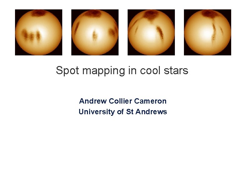
Spot mapping in cool stars Andrew Collier Cameron

Spot mapping in cool stars Andrew Collier Cameron University of St Andrews

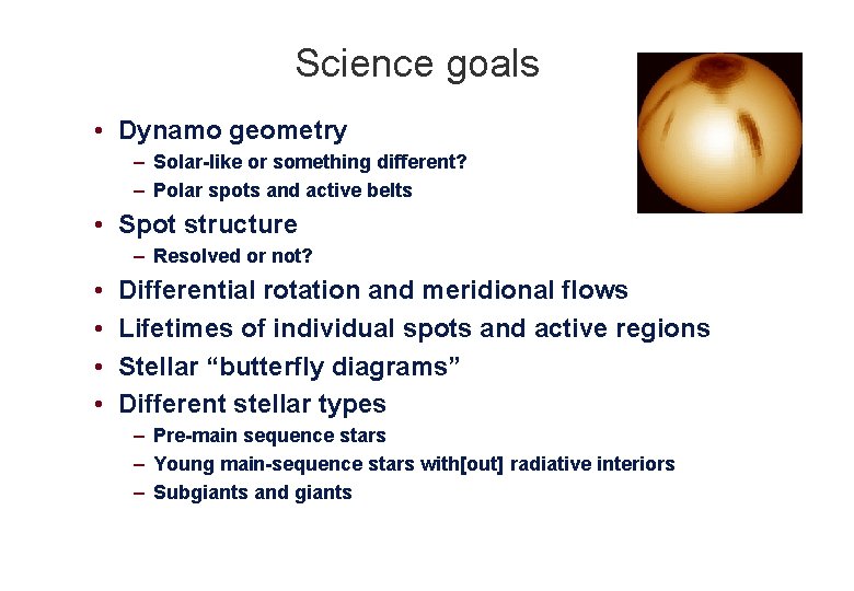
Science goals • Dynamo geometry – Solar-like or something different? – Polar spots and active belts • Spot structure – Resolved or not? • • Differential rotation and meridional flows Lifetimes of individual spots and active regions Stellar “butterfly diagrams” Different stellar types – Pre-main sequence stars – Young main-sequence stars with[out] radiative interiors – Subgiants and giants

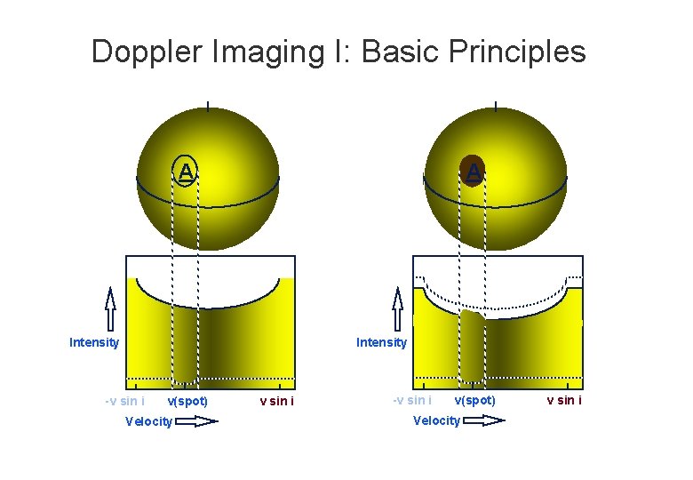
Doppler Imaging I: Basic Principles A A Intensity -v sin i v(spot) Velocity v sin i

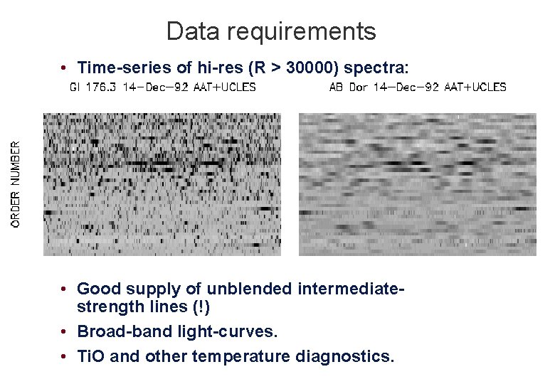
Data requirements • Time-series of hi-res (R > 30000) spectra: • Good supply of unblended intermediatestrength lines (!) • Broad-band light-curves. • Ti. O and other temperature diagnostics.

• Rotational broadening gives shallow, blended lines … • … but LTE models yield estimates of their positions and strengths

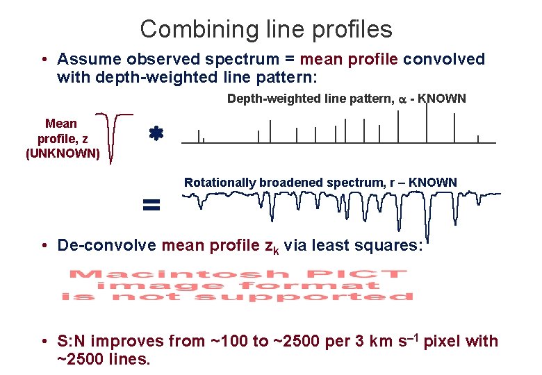
Combining line profiles • Assume observed spectrum = mean profile convolved with depth-weighted line pattern: Depth-weighted line pattern, - KNOWN Mean profile, z (UNKNOWN) = Rotationally broadened spectrum, r – KNOWN • De-convolve mean profile zk via least squares: • S: N improves from ~100 to ~2500 per 3 km s– 1 pixel with ~2500 lines.

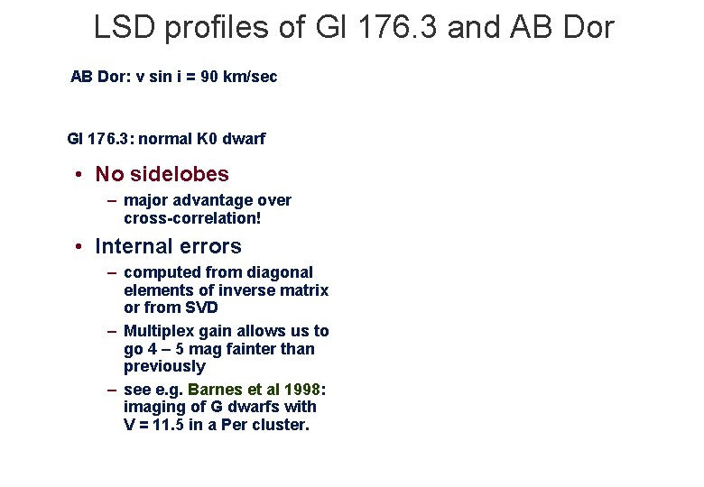
LSD profiles of Gl 176. 3 and AB Dor: v sin i = 90 km/sec Gl 176. 3: normal K 0 dwarf • No sidelobes – major advantage over cross-correlation! • Internal errors – computed from diagonal elements of inverse matrix or from SVD – Multiplex gain allows us to go 4 – 5 mag fainter than previously – see e. g. Barnes et al 1998: imaging of G dwarfs with V = 11. 5 in a Per cluster.

Time series: deconvolved Stokes I profiles • AB Dor • 1996 Dec 23 -29 • AAT + UCLES +Semel polarimeter • Sum of L & R circularly polarized line profiles

Choice of mapping parameter • What are we trying to map on the stellar surface? • Temperature: f ~ T 4 – – – Bolometric surface brightness Form of spectrum varies continuously with f No restriction on mix of bright and dark features Needs grid of (synthetic) spectra May give problems in blurred images of unresolved spots • Spot filling factor: – – f = Aspots / (Aspots + Aphot) Takes values 0 < f < 1 Requires fixed photospheric and spot temperatures Doesn’t allow other temperature components Can use “template” spectra of real stars with appropriate Teff to represent “spot” and “photosphere” – Copes well with unresolved spots

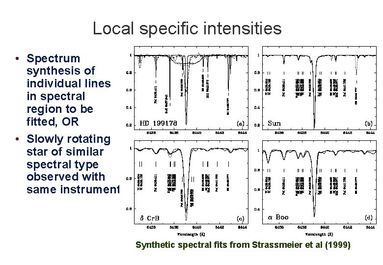
Local specific intensities • Spectrum synthesis of individual lines in spectral region to be fitted, OR • Slowly rotating star of similar spectral type observed with same instrument. Synthetic spectral fits from Strassmeier et al (1999)

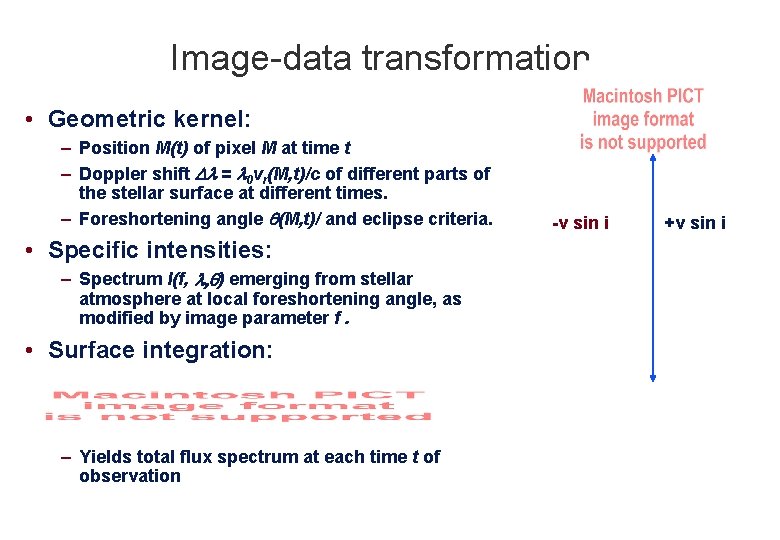
Image-data transformation • Geometric kernel: – Position M(t) of pixel M at time t – Doppler shift Dl = l 0 vr(M, t)/c of different parts of the stellar surface at different times. – Foreshortening angle q(M, t)/ and eclipse criteria. • Specific intensities: – Spectrum I(f, l, q) emerging from stellar atmosphere at local foreshortening angle, as modified by image parameter f. • Surface integration: – Yields total flux spectrum at each time t of observation -v sin i +v sin i

Regularised least-squares solutions

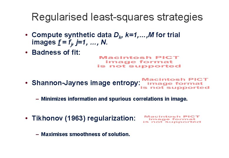
Regularised least-squares strategies • Compute synthetic data Dk, k=1, …, M for trial images f = fj, j=1, …, N. • Badness of fit: • Shannon-Jaynes image entropy: – Minimizes information and spurious correlations in image. • Tikhonov (1963) regularization: – Maximises smoothness of solution.

RX J 1508. 6 -4423 • Deconvolved profiles and fitted model with unspotted profile subtracted. Data (From Donati et al 2000) Model fit Residuals

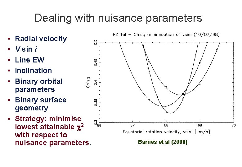
Dealing with nuisance parameters • • • Radial velocity V sin i Line EW Inclination Binary orbital parameters • Binary surface geometry • Strategy: minimise lowest attainable c 2 with respect to nuisance parameters. Barnes et al (2000)

A more systematic approach • Hendry & Mochnacki Ap. J 531, 467 (2000) : – Surface imaging of contact binary VW Cep – Nuisance parameters adjusted simultaneously with image: » Phase correction Df » Velocity amplitude K » System centre-of-mass velocity g » Inclination i » Mass ratio q » Fill-out factor F » Unspotted primary Teff – Artefacts introduced by bad nuisanceparameter values decrease final image entropy. VW Cep, 1991 Mar to 1993 May

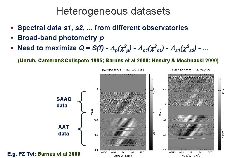
Heterogeneous datasets • Spectral data s 1, s 2, . . . from different observatories • Broad-band photometry p • Need to maximize Q = S(f) - Lp(c 2 p) - Ls 1(c 2 s 1) - Ls 1(c 2 s 2) -. . . (Unruh, Cameron&Cutispoto 1995; Barnes et al 2000; Hendry & Mochnacki 2000) SAAO data AAT data E. g. PZ Tel: Barnes et al 2000

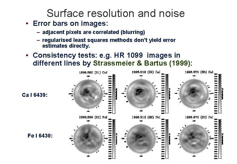
Surface resolution and noise • Error bars on images: – adjacent pixels are correlated (blurring) – regularised least squares methods don’t yield error estimates directly. • Consistency tests: e. g. HR 1099 images in different lines by Strassmeier & Bartus (1999): Ca I 6439: Fe I 6430:

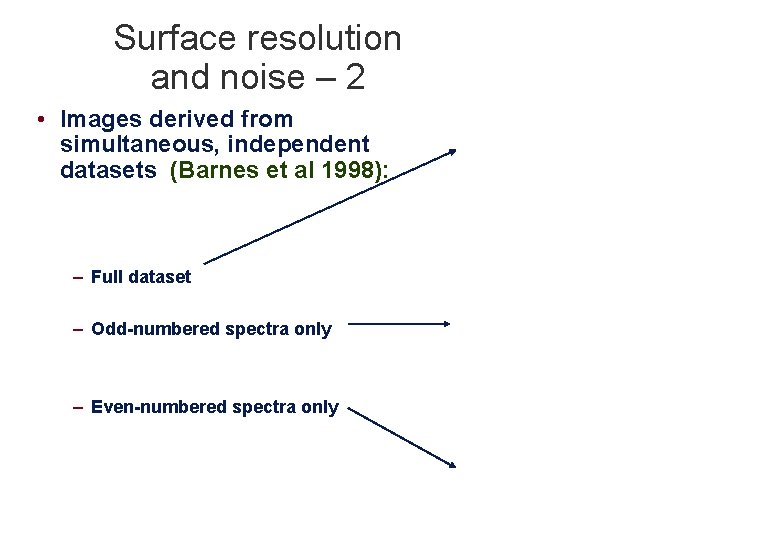
Surface resolution and noise – 2 • Images derived from simultaneous, independent datasets (Barnes et al 1998): – Full dataset – Odd-numbered spectra only – Even-numbered spectra only

The Occamian approach • Applied to spot imaging problem by Berdyugina (1998) – Astron. Astrophys. 338, 97– 105 (1998) • Matrix P defines “PSF” of forward problem: • Approximation to Hessian matrix: • Eigenvectors of H define principal axes of error ellipsoid in image space. • Principal components with small eigenvalues are poorly-constrained by data • A subset of those principle components exhausts the information content of image f • Use SVD to solve for f; error estimates are:

Future prospects: The perfect spot code • The perfect code would have: – Simultaneous fitting of nuisance parameters – Error bars on images and nuisance parameters – Full utilisation of temperature-dependent profile information in thousands of lines – Correct treatment of heterogeneous data types (spectra, photometry, Ti. O, . . . ) • The perfect user of such a code would: – Use well-understood statistical methods to test hypotheses (c 2 rules OK!) – Perform these tests in data space where errors are understood! – Always remember the First Law of Doppler Imaging: – If you can’t see it in the trailed spectrum, it probably isn’t there. -v sin i +v sin i

Starspots as flow tracers • Latitude-dependent rotation in 3 images of AB Dor (AAT 1996 Dec 23– 29, Donati et al 1999)

Surface shear: 1996 December 23 - 29 • CCF for surfacebrightness images Equator pulls one rotation ahead of polar regions every ~ 120 d or so -- very similar to solar shear! • CCF for magnetic images:

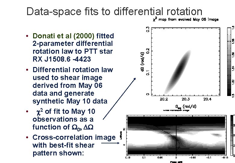
Data-space fits to differential rotation • Donati et al (2000) fitted 2 -parameter differential rotation law to PTT star RX J 1508. 6 -4423 • Differential rotation law used to shear image derived from May 06 data and generate synthetic May 10 data • c 2 of fit to May 10 observations as a function of W 0, DW • Cross-correlation image with best-fit shear pattern shown:

Spot lifetimes: dwarfs vs (sub)giants • Barnes et al (1998): No correlation of fine-scale spot structure between 2 images of Per G dwarf He 699 taken 1 month apart. – But overall active-region positions unchanged? • Berdyugina et al (1999): Major spot complexes on II Peg persist for 2 -3 months, but fine structure unresolved. 1997: June August December July October November 1998:

Do spots drift poleward on HR 1099? • Strassmeier & Bartus 1999 • Spectra on 57 consecutive nights, 1996 Nov-Dec • Movie constructed from “running mean” sequences of 12 consecutive spectra. • Main spot and transient neighbours form and dissolve on timescales consistent with Berdyugina et al’s II Peg maps: Latitude Polar view Longitude

So how far have we got? • Differential rotation: – Young solar-type stars have solar-like latitudinal shear even at rotation rates 50 times solar. – Study of meridional flows needs better-sampled data over timescales of weeks to months. • Lifetimes of individual spots and active regions – Weeks to months (respectively? ) • Stellar cycles and “butterfly diagrams” – Wait for Jean-François Donati’s talk! • Different stellar types – Pre-main sequence stars -- more needed – Young main-sequence stars -- well studied, but what do fully-convective M dwarfs look like? – Subgiants and giants -- longer-lived spots? – Binaries -- the next big challenge.