Simulation packages and Review of Codes Alexej Grudiev

Simulation packages and Review of Codes Alexej Grudiev CERN, BE-RF

Packages for computer simulations of electromagnetic EM fields and more CST Gdfid. L ACE 3 P HFSS COMSOL

CST Studio Suite CST STUDIO SUITE: - CST MWS - CST DS - CST EMS - CST PS - CST MPS - CST PCBS - CST CS - CST MICROSTRIPES - Antenna Magus

CST: All(? ) you need in one package • Powerful and user-friendly Input: • Probably the best time domain (TD) solver for wakefields or beam coupling impedance calculations (MAFIA) • Beta < 1 • Finite Conductivity walls • Once geometry input is done it can be used both for TD and FD simulations • Moreover using Design Studio (DS) it can be combined with the other studios for multiphysics and integrated electronincs simulation, but this is relatively fresh fields of expertise for CST • Accelerator physics oriented post processor, especially in MWS and PS • Enormous progress over the last few years compared to the competitors. Courtesy of Igor Syratchev An example of what can be solved easily on a standard PC

CST (examples) Two examples of what can be solved on bigger PC: 128 GB of RAM and 24 CPUs CLIC accelerating structure from Cu with HOM damping loads from Si. C (frequency dependent properties) Giovanni De Michele

Wx [V/p. C] CST (examples) Transverse wake at offset of 0. 5 mm Zx [Ω] s [mm] Transverse beam couping impedance at offset of 0. 5 mm f [GHz]

CST (examples) LHC TDI 5 m long with ferrite Benoit Salvant

CST MWS: Comparison with HFSS (Praveen Ambattu, Vasim F. Khan) Property MWS (PEC) HFSS (Cu) Freq, GHz 11. 9941 11. 9959 QCu 6395 6106 Rt/Q, Ohm 54. 65 53. 78 Esurf/Et 3. 43 3. 28 Hsurf/Et 0. 0114 0. 0106 Mesh view MWS HFSS • MWS used Perfect Boundary Approximation, 134, 912 hexahedra per quarter (lines/lamda=40, lower mesh limit=40, mesh line ratio limit=40) • HFSS used 8, 223 tetrahedra per quarter (surface approximation= 5 mm, aspect ratio=5)

CST MWS: Example. S-parameters in CLIC Crab cavity Mesh view (Praveen Ambattu)

CST: Shortcomings 1. Cartesian mesh: Especially in FD can results to less accurate calculations of frequency, Q-factor, surface fields compared to tetrahedral mesh (HFSS, COMSOL, ACE 3 P). Tetrahedral mesh became available only recently but it is improving very rapidly. 2. Boundary conditions can be set only in Cartesian planes 3. No Field Calculator (HFSS) 4. From three eigenmode solvers only one takes into account losses but it is iterative and very slow 5. . With a great help of Andrei Lunin

HFSS: Still an excellent tool for FD High-Performance Electronic Design Ansoft Designer ANSYS HFSS ANSYS Q 3 D Extractor ANSYS SIwave ANSYS TPA Electromechanical Design ANSYS Multiphysics ANSYS Maxwell ANSYS Simplorer ANSYS PExprt ANSYS RMxprt Product options Ansoft. Links for ECAD Ansoft. Links for MCAD ANSYS Distributed Solve ANSYS Full-Wave SPICE ANSYS Optimetrics ANSYS Par. ICs • HFSS was and I think still is superior tool for FD simulations both S-pars and eigenmode, though CST shows significant progress in the recent years • Automatic generation and refinement of tetrahedral mesh • Most complete list of boundary conditions which can be applied on any surface • Ansoft Designer allows to co-simulate the pickup (antenna), cables plus electronics and together with versatile Optimetrics optimise the design of the whole device • Last year HFSS become a integral part of ANSYS – reference tool for thermo-mechanical simulations -> multiphysics • Last year time-dependent solver has been released

HFSS (examples, eigenmode) LHC TDI 5 m long beam dump: One of the most dangerous eigenmodes at 1. 227 GHz, Q = 873, Tetrahedral mesh with mixed order (0 th , 1 st , 2 nd) elements: Ntetr = 1404891 Solution obtained on a workstation with 128 GB of RAM,

HFSS (example, S-parameters) Incident plane wave excitation Port excitation O. Kononenko Inverse FFT

HFSS example

HFSS: shortcomings 1. No possibility to simulate particles 2. Automatic mesh is not always perfect, but it has improved after adoption by ANSYS 3. TD and multiphysics are only recently implemented, but thermo-mechanics from ANSYS is a reference by itself 4. .

Gdfid. L: Parallel and easy to use tool bruns@gdfidl. de The Gdfid. L Electromagnetic Field simulator Gdfid. L computes electromagnetic fields in 3 D-structures using parallel or scalar computers. Gdfid. L computes • Time dependent fields in lossfree or lossy structures. The fields may be excited by • port modes, • relativistic line charges. • Resonant fields in lossfree or lossy structures. • The postprocessor computes from these results eg. Scattering parameters, wake potentials, Q-values and shunt impedances. Features • Gdfid. L computes only in the field carrying parts of the computational volume. For eg. waveguide systems, this makes Gdfid. L about three to ten times faster than other Finite Difference based programs. • Gdfid. L uses generalised diagonal fillings to approximate the material distribution. This reduces eg. the frequency error by about a factor of ten. • For eigenvalue computations, Gdfid. L allows periodic boundary conditions in all three cartesian directions simultaneously. • Gdfid. L runs on parallel and serial computers. Gdfid. L also runs on clusters of workstations. Availability • Gdfid. L only runs on UNIX-like operating systems. Price The price for a one year license for the serial version of Gdfid. L (including support) starts at 10. 000 Euro. The price for a one year license for the parallel versions starts at 20. 000 Euro. Access to a powerful cluster where Gdfid. L is installed on costs 9. 000 Euro per year. Powerful Syntax Material Approximation Absorbing Boundary Conditions Periodic Boundary Conditions

Gdfid. L (example) CLIC accelerating structure from Cu with HOM damping loads from Si. C (frequency dependent properties)

Gdfid. L: shortcomings 1. 2. 3. 4. Available only under UNIX-like systems Geometry input is limited It is ‘one man show’. . .

COMSOL: pioneer in multiphysics COMSOL Multiphysics® AC/DC Module Heat Transfer Module CFD Module Chemical Reaction Engineering Module Optimization Module® Live. Link™ for MATLAB® CAD Import Module RF Module Structural Mechanics Module Microfluidics Module Batteries & Fuel Cells Module Material Library Live. Link™ for Solid. Works® Live. Link™ for Space. Claim® MEMS Module Geomechanics Module Subsurface Flow Module Electrodepositi on Module Particle Tracing Module Live. Link™ for Pro/ENGINEER Live. Link™ for Creo™ Parametric Plasma Module Acoustics Module Live. Link™ for Inventor® Live. Link™ for Auto. CAD® ®

COMSOL: example df/dp Calculation Electromagnetic Waves • Solving only for the RF domain • Applying the prober boundary conditions Solid Mechanics • Solving only for the Cavity Vessel • Applying the proper fixed constraints, symmetries, displacements, and boundary load Three Multiphysic Modules Moving Mesh • Solving for all domains • Applying the proper prescribed and free mesh deformation/displacement EM • Eigen frequency simulation to find the resonant frequency (f 0) Solid • Find the deformation under given pressure load (PL) Mechanics Two Simulation Studies Moving Mesh Study 1 Study 2 • Eigen-frequency (to find f 0) • Stationary (solving only for solid mechanics and moving mesh) • Eigen-frequency (to find f p) Mohamed Hassan EM • Update the mesh after deformation • Eigen frequency simulation to find the resonant frequency after deformation (fp)

Stainless Steel Vessel Mohamed Hassan Example PEC Electromagnetic Waves RF Domain Niobium Shell PMC • Solving only for the RF domain • Applying the prober boundary conditions Symmetry Boundaries Fixed Constraint Solid Mechanics • Solving only for the Cavity Vessel • Applying the proper fixed constraints, symmetries, displacements, and boundary load Moving Mesh =0 dx Prescribed Displacement u, v, w Pressure Boundary Load 0 Prescribed dy = Displacement dx dz=0 • Solving for all domains • Applying the proper prescribed and free mesh deformation/displacement Prescribed Deformation u, v, w Free Deformation

COMSOL: example Meshes used for RF kick simulations : a ) HFSS , b ) CST MWS, c) COMSOL a) b) c) A. Lunin, et. al. , FINAL RESULTS ON RF AND WAKE KICKS CAUSED BY THE COUPLERS FOR THE ILC CAVITY, IPAC 10, Kyoto, Japan • ‘Highly regularized tetrahedral mesh can be built by versatile COMSOL mesh generator’ • ‘Well parallelized, direct method for eigenmode calculations with losses and smooth surface fields’ Andrei Lunin

COMSOL: shortcomings • Geometry input is limited • Port excitation mode description is not convenient • S-parameter solver is not convenient • Postprocessing is not well developed at least for what concerns accelerator physicists and engineers Andrei Lunin

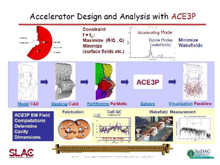
ACE 3 P

waveguide ACE 3 P: example CLIC two-beam module rf circuit AS AS PETS Arno Candel et. al. , SLAC-PUB-14439

ACE 3 P: shortcomings • Very complex package to use. It is not userfriendly at all and requires a lots of time to invest before it can be used efficiently • It is not a commercial product -> no manual reference, limited tech support. No it is an open source. • . . .

Summary 1. CST Larger objects in TD 2. Better FD calculations, 3 D EM + circuit co-simulation, RF + thermal + structural More multiphysics ANSYS HFSS COMSOL Gdfid. L Accurate solution for very larger objects in TD and FD 3. ACE 3 P