Simulated Annealing Premchand Akella Agenda Motivation The algorithm

Simulated Annealing Premchand Akella

Agenda • • • Motivation The algorithm Its applications Examples Conclusion

Introduction • Various algorithms proposed for placement in circuits. • Constructive placement vs Iterative improvement. • Simulated Annealing – an iterative improvement algorithm.

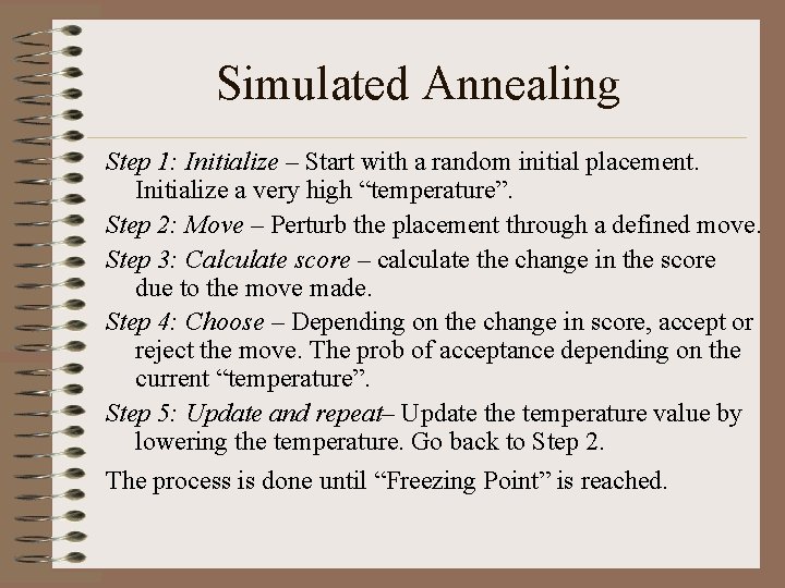
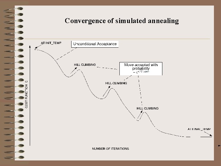
Motivation • Annealing in metals • Heat the solid state metal to a high temperature • Cool it down very slowly according to a specific schedule. • If the heating temperature is sufficiently high to ensure random state and the cooling process is slow enough to ensure thermal equilibrium, then the atoms will place themselves in a pattern that corresponds to the global energy minimum of a perfect crystal.

Simulated Annealing Step 1: Initialize – Start with a random initial placement. Initialize a very high “temperature”. Step 2: Move – Perturb the placement through a defined move. Step 3: Calculate score – calculate the change in the score due to the move made. Step 4: Choose – Depending on the change in score, accept or reject the move. The prob of acceptance depending on the current “temperature”. Step 5: Update and repeat– Update the temperature value by lowering the temperature. Go back to Step 2. The process is done until “Freezing Point” is reached.

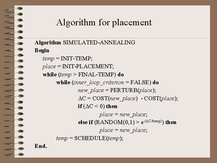
Algorithm for placement Algorithm SIMULATED-ANNEALING Begin temp = INIT-TEMP; place = INIT-PLACEMENT; while (temp > FINAL-TEMP) do while (inner_loop_criterion = FALSE) do new_place = PERTURB(place); ΔC = COST(new_place) - COST(place); if (ΔC < 0) then place = new_place; else if (RANDOM(0, 1) > e-(ΔC/temp)) then place = new_place; temp = SCHEDULE(temp); End.

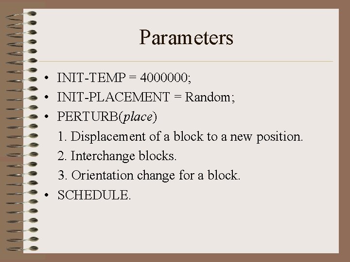
Parameters • INIT-TEMP = 4000000; • INIT-PLACEMENT = Random; • PERTURB(place) 1. Displacement of a block to a new position. 2. Interchange blocks. 3. Orientation change for a block. • SCHEDULE.

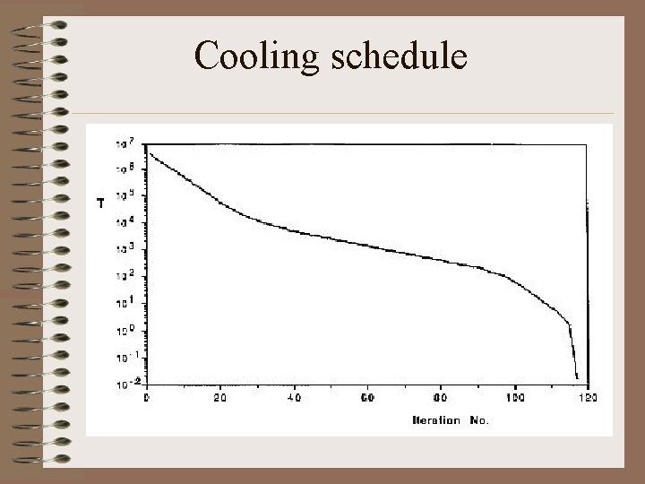
Cooling schedule

Convergence of simulated annealing

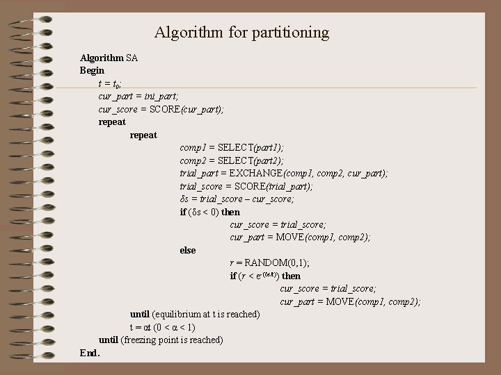
Algorithm for partitioning Algorithm SA Begin t = t 0; cur_part = ini_part; cur_score = SCORE(cur_part); repeat comp 1 = SELECT(part 1); comp 2 = SELECT(part 2); trial_part = EXCHANGE(comp 1, comp 2, cur_part); trial_score = SCORE(trial_part); δs = trial_score – cur_score; if (δs < 0) then cur_score = trial_score; cur_part = MOVE(comp 1, comp 2); else r = RANDOM(0, 1); if (r < e-(δs/t)) then cur_score = trial_score; cur_part = MOVE(comp 1, comp 2); until (equilibrium at t is reached) t = αt (0 < α < 1) until (freezing point is reached) End.

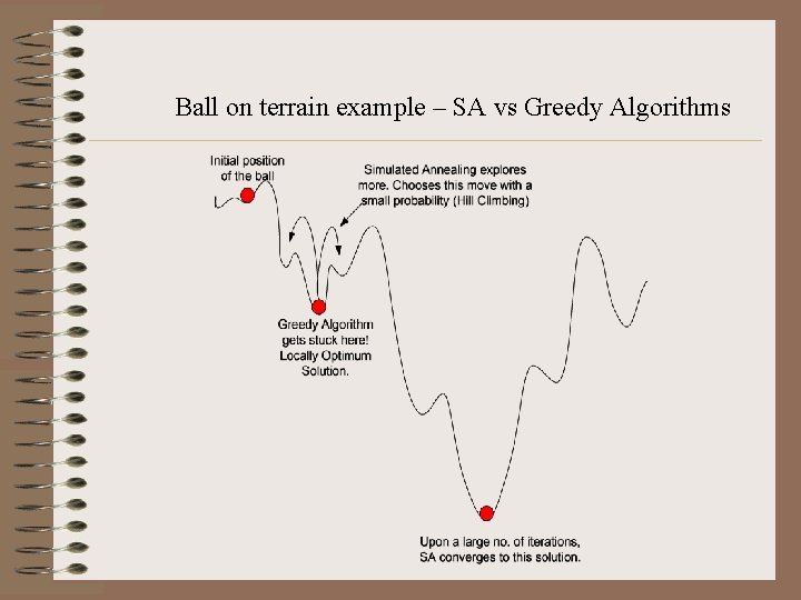
Qualitative Analysis • • • Randomized local search. Is simulated annealing greedy? Controlled greed. Once-a-while exploration. Is a greedy algorithm better? Where is the difference? • The ball-on-terrain example.

Ball on terrain example – Simulated Annealing vs Greedy Algorithms The ball is initially placed at a random position on the terrain. From the current position, the ball should be fired such that it can only move one step left or right. What algorithm should we follow for the ball to finally settle at the lowest point on the terrain?

Ball on terrain example – SA vs Greedy Algorithms

Applications • Circuit partitioning and placement. • Strategy scheduling for capital products with complex product structure. • Umpire scheduling in US Open Tennis tournament! • Event-based learning situations.

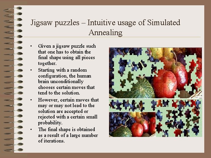
Jigsaw puzzles – Intuitive usage of Simulated Annealing • • Given a jigsaw puzzle such that one has to obtain the final shape using all pieces together. Starting with a random configuration, the human brain unconditionally chooses certain moves that tend to the solution. However, certain moves that may or may not lead to the solution are accepted or rejected with a certain small probability. The final shape is obtained as a result of a large number of iterations.

Conclusions • Simulated Annealing algorithms are usually better than greedy algorithms, when it comes to problems that have numerous locally optimum solutions. • Simulated Annealing is not the best solution to circuit partitioning or placement. Network flow approach to solving these problems functions much faster. • Simulated Annealing guarantees a convergence upon running sufficiently large number of iterations.

Thank You!