Heuristic Optimization Methods Lecture 03 Simulated Annealing Simulated

Heuristic Optimization Methods Lecture 03 – Simulated Annealing

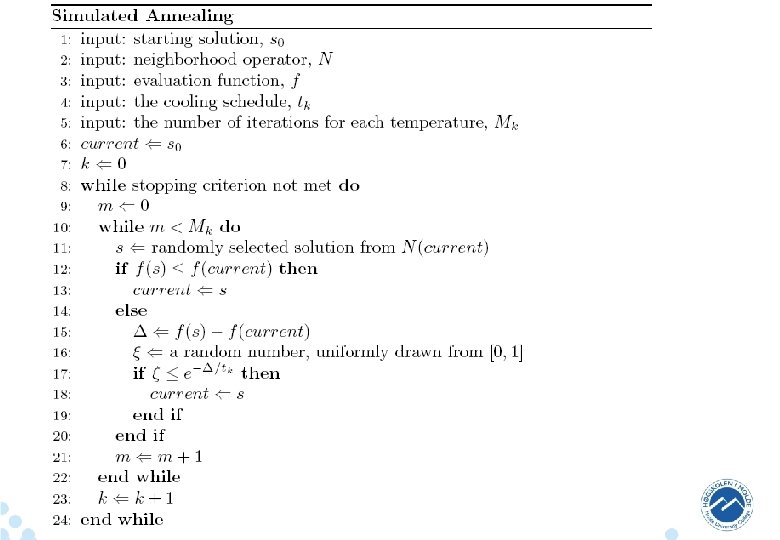
Simulated Annealing • A metaheuristic inspired by statistical thermodynamics – Based on an analogy with the cooling of material in a heat bath • • Used in optimization for 20 years Very simple to implement A lot of literature Converges to the global optimum under weak assumptions (- usually slowly) 2

Simulated Annealing - SA • Metropolis’ algorithm (1953) – Algorithm to simulate energy changes in physical systems when cooling • Kirkpatrick, Gelatt and Vecchi (1983) – Suggested to use the same type of simulation to look for good solutions in a COP 3

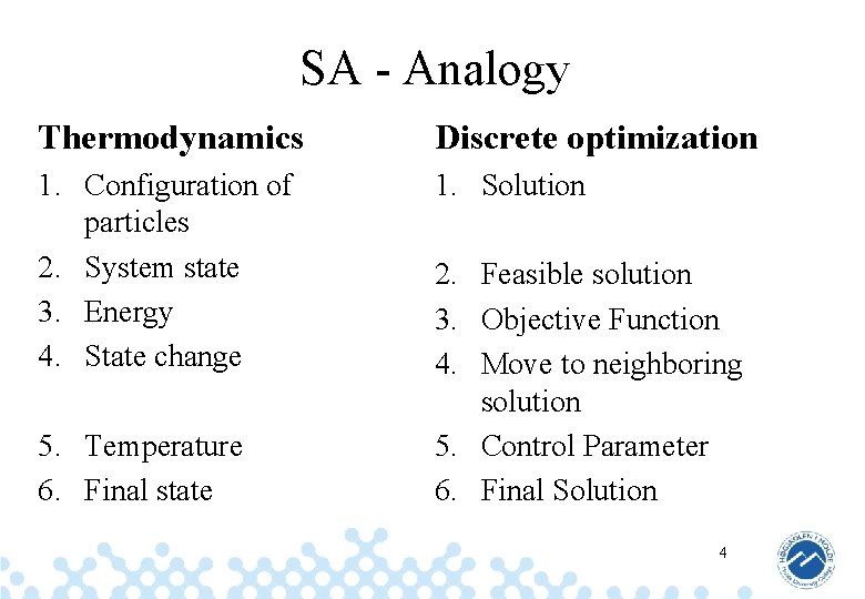
SA - Analogy Thermodynamics Discrete optimization 1. Configuration of particles 2. System state 3. Energy 4. State change 1. Solution 5. Temperature 6. Final state 2. Feasible solution 3. Objective Function 4. Move to neighboring solution 5. Control Parameter 6. Final Solution 4

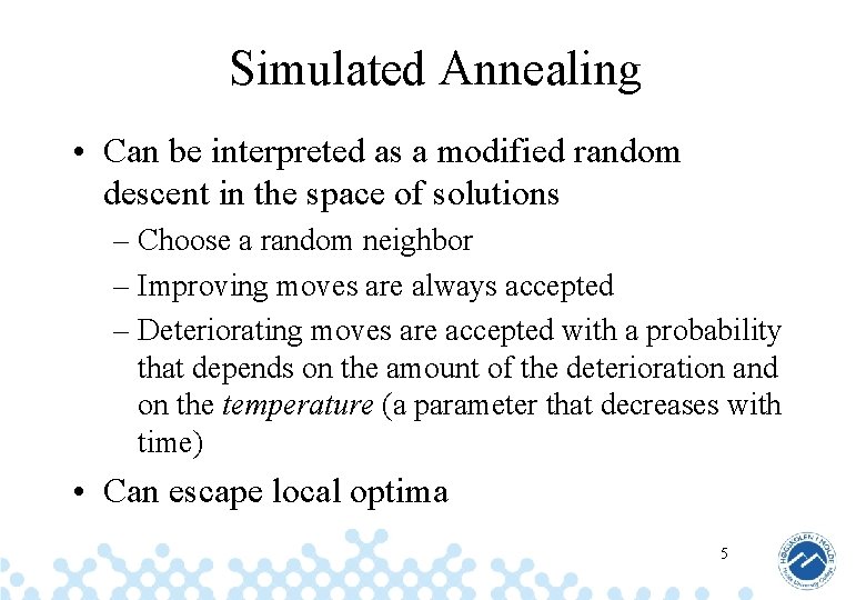
Simulated Annealing • Can be interpreted as a modified random descent in the space of solutions – Choose a random neighbor – Improving moves are always accepted – Deteriorating moves are accepted with a probability that depends on the amount of the deterioration and on the temperature (a parameter that decreases with time) • Can escape local optima 5

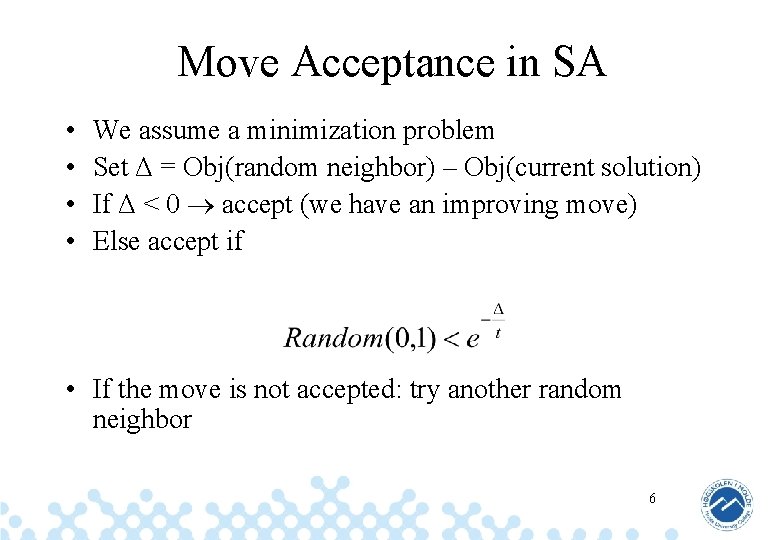
Move Acceptance in SA • • We assume a minimization problem Set Δ = Obj(random neighbor) – Obj(current solution) If Δ < 0 accept (we have an improving move) Else accept if • If the move is not accepted: try another random neighbor 6

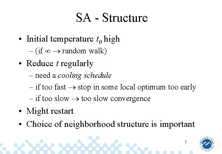
SA - Structure • Initial temperature t 0 high – (if random walk) • Reduce t regularly – need a cooling schedule – if too fast stop in some local optimum too early – if too slow convergence • Might restart • Choice of neighborhood structure is important 7

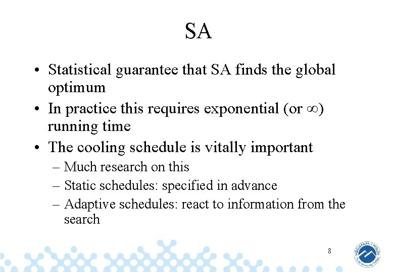
SA • Statistical guarantee that SA finds the global optimum • In practice this requires exponential (or ) running time • The cooling schedule is vitally important – Much research on this – Static schedules: specified in advance – Adaptive schedules: react to information from the search 8

9

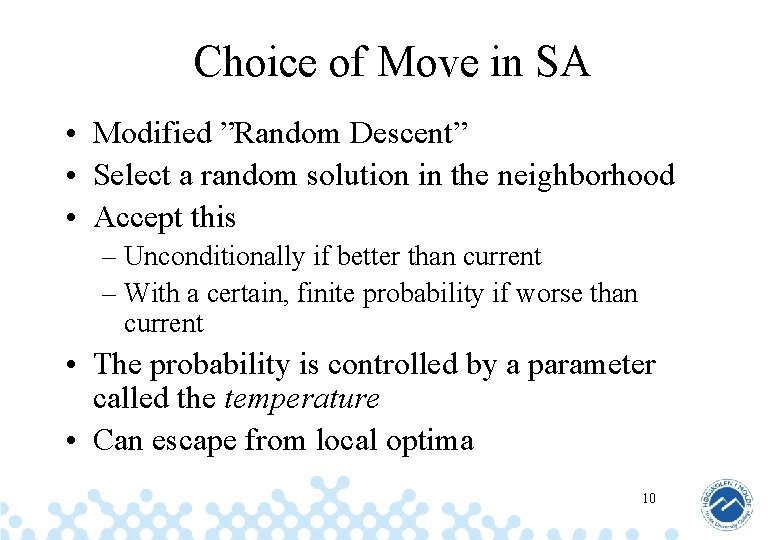
Choice of Move in SA • Modified ”Random Descent” • Select a random solution in the neighborhood • Accept this – Unconditionally if better than current – With a certain, finite probability if worse than current • The probability is controlled by a parameter called the temperature • Can escape from local optima 10

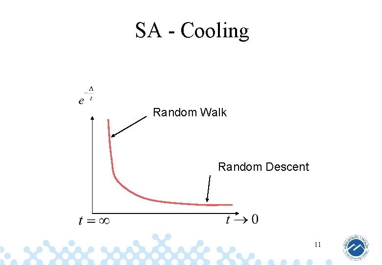
SA - Cooling Random Walk Random Descent 11

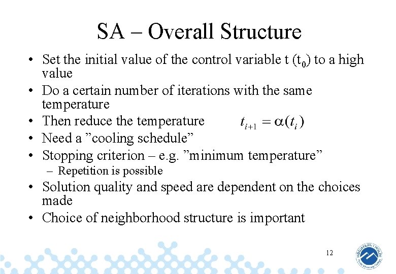
SA – Overall Structure • Set the initial value of the control variable t (t 0) to a high value • Do a certain number of iterations with the same temperature • Then reduce the temperature • Need a ”cooling schedule” • Stopping criterion – e. g. ”minimum temperature” – Repetition is possible • Solution quality and speed are dependent on the choices made • Choice of neighborhood structure is important 12

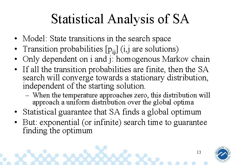
Statistical Analysis of SA • • Model: State transitions in the search space Transition probabilities [pij] (i, j are solutions) Only dependent on i and j: homogenous Markov chain If all the transition probabilities are finite, then the SA search will converge towards a stationary distribution, independent of the starting solution. – When the temperature approaches zero, this distribution will approach a uniform distribution over the global optima • Statistical guarantee that SA finds a global optimum • But: exponential (or infinite) search time to guarantee finding the optimum 13

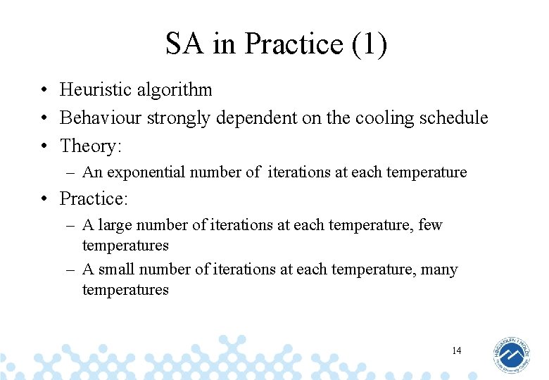
SA in Practice (1) • Heuristic algorithm • Behaviour strongly dependent on the cooling schedule • Theory: – An exponential number of iterations at each temperature • Practice: – A large number of iterations at each temperature, few temperatures – A small number of iterations at each temperature, many temperatures 14

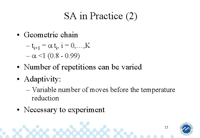
SA in Practice (2) • Geometric chain – ti+1 = ti, i = 0, …, K – <1 (0. 8 - 0. 99) • Number of repetitions can be varied • Adaptivity: – Variable number of moves before the temperature reduction • Necessary to experiment 15

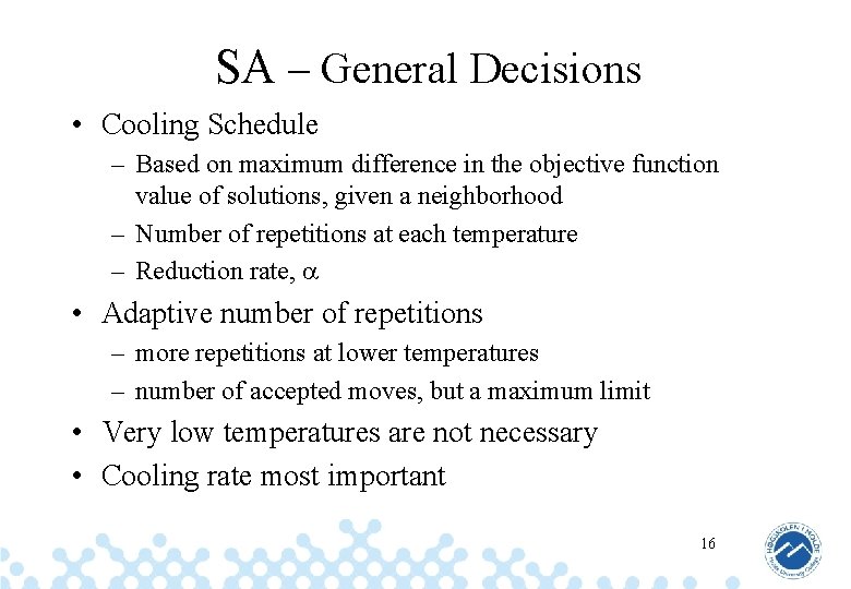
SA – General Decisions • Cooling Schedule – Based on maximum difference in the objective function value of solutions, given a neighborhood – Number of repetitions at each temperature – Reduction rate, • Adaptive number of repetitions – more repetitions at lower temperatures – number of accepted moves, but a maximum limit • Very low temperatures are not necessary • Cooling rate most important 16

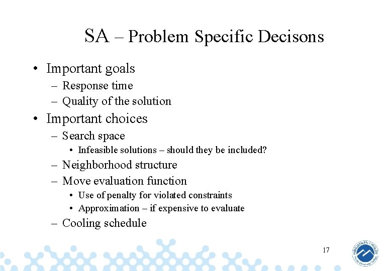
SA – Problem Specific Decisons • Important goals – Response time – Quality of the solution • Important choices – Search space • Infeasible solutions – should they be included? – Neighborhood structure – Move evaluation function • Use of penalty for violated constraints • Approximation – if expensive to evaluate – Cooling schedule 17

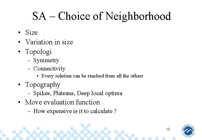
SA – Choice of Neighborhood • Size • Variation in size • Topologi – Symmetry – Connectivity • Every solution can be reached from all the others • Topography – Spikes, Plateaus, Deep local optima • Move evaluation function – How expensive is it to calculate ? 18

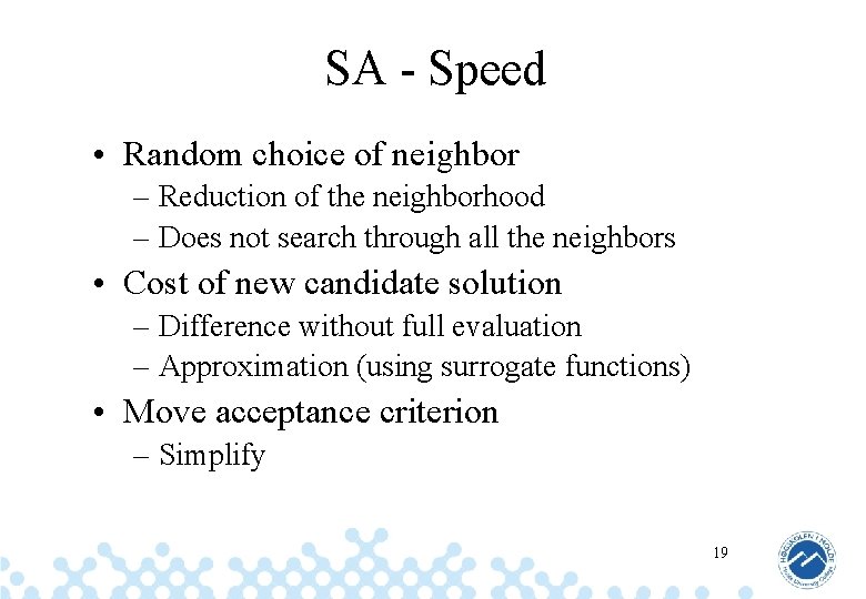
SA - Speed • Random choice of neighbor – Reduction of the neighborhood – Does not search through all the neighbors • Cost of new candidate solution – Difference without full evaluation – Approximation (using surrogate functions) • Move acceptance criterion – Simplify 19

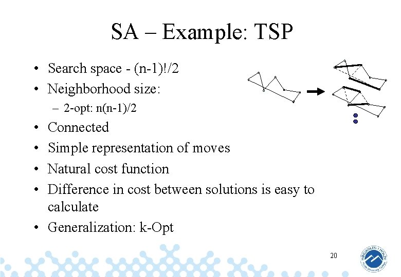
SA – Example: TSP • Search space - (n-1)!/2 • Neighborhood size: – 2 -opt: n(n-1)/2 • • Connected Simple representation of moves Natural cost function Difference in cost between solutions is easy to calculate • Generalization: k-Opt 20

SA – Fine Tuning • • Test problems Test bench Visualization of solutions Values for – – cost / penalties temperature number / proportion of accepted move iterations / CPU time • Depencies between the SA-parameters • The danger of overfitting 21

SA – Summary • Inspired by statistical mechanics - cooling • Metaheuristic – Local search – Random descent – Use randomness to escape local optima • Simple and robust method – Easy to get started • Proof for convergence to the global optimum – Worse than complete search • In practise: – Computationally expensive – Fine tuning can give good results – SA can be good where robust heuristics based on problem structure are difficult to make 22

Topics for the next Lecture • More Local Search based metaheuristics – – – Simulated Annealing (the rest) Threshold Accepting Variable Neighborhood Search Iterative Local Search Guided Local Search • This will prepare the ground for more advanced mechanisms, such as found in – Tabu Search – Adaptive Memory Procedures 23