Simulated Annealing R W Eglese Simulated Annealing A

Simulated Annealing R. W. Eglese, “Simulated Annealing: A tool for Operational Research, ” European Journal of Operational Research 46 (1990) 271 -281 Presented by P. L. Chiu 1

Outline n n Simulated Annealing Example P. L. Chiu 2

Introduction n n SA can be considered as one type of randomized heuristic for combinatorial optimization problems. Many combinatorial optimization problems have been shown to be NP-hard. n n The running time for any algorithms currently known to guarantee an optimal solution is an exponential function of the size of the problem. Simulated Annealing (SA) is a method for obtaining good solutions to difficult optimization problems. P. L. Chiu 3

Introduction n SA is not the only heuristic search method to have received attention recently. n Genetic algorithms n Neural networks n Tabu search n Target analysis P. L. Chiu 4

Introduction n n SA is one of many heuristic approaches designed to give a good though not necessarily optimal solution, within a reasonable computing time. SA has also been extended to optimization problems for continuous variables. P. L. Chiu 5

The Physical Analogy n n n Refer to the process of finding low energy states of a solid by initially melting the substance, and then lowing the temperature slowly, spending a long time at temperatures closely to the freezing point. In a liquid, the particles are arranged randomly. The ground state of the solid n corresponds to the minimum energy configuration, will have a particular structure, such as seen in a crystal. P. L. Chiu 6

The Physical Analogy n n n metastable n If the cooling is not done slowly, the resulting solid will be frozen into a metastable, locally optimal structure, such as a glass or a crystal with several defects in the structure. The different states of the substance correspond to different feasible solutions to the combinatorial optimization problem. n Ground state global optimal solutions n Metastable local optimal; feasible solutions The energy of the system corresponds to the function to be minimized. P. L. Chiu 7

The Physical Analogy n Thermal equilibrium n n The probability distribution of the system states follows a Boltzmann distribution or T: temperature Ei: energy of state i Z(T): the partition function required for normalization P. L. Chiu 8

Theoretical Results n n n n If the temperature T is kept constant, then the transition matrix, Pij , is independent of the iteration number. Correspond to a homogeneous Markov chain The stationary distribution q(i) , corresponds to Boltzmann distribution. The limit as T→ 0 of this stationary distribution is a uniform distribution over set of optimal solutions. The SA algorithm converges to the set of globally optimal solutions. But this result does not tell us anything about the number of iterations required to achieve convergence. P. L. Chiu 9

n n n n 1. Select an objective function E(x); 2. Select an initial temperature T>0; 3. Set temperature change counter t=0; 4. Repeat 4. 1 Set repetition counter n=0; 4. 2 Repeat 4. 2. 1 Generate state xi+1, a neighbor of xi; 4. 2. 2 Calculate E=E(xi+1) E(xi); 4. 2. 3 If E<0 then xi=xi+1; 4. 2. 4 else if random(0, 1)<exp( E/T) then xi=xi+1; 4. 2. 5 n=n+1; 4. 3 Until n=r(t); 4. 4 t=t+1; 4. 5 T=T(t); Until stopping criterion true. P. L. Chiu 13

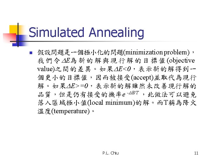
Description of SA n Acceptance function n n the probability of accepting: exp(- E/T) T is a control parameter which corresponds to temperature in the analogy with physical annealing. Small increase in f ( E is small)are more likely to be accepted than large increase. When T is high most moves will be accepted, but as T approaches zero most uphill moves will be rejected. P. L. Chiu 14

Cooling Schedule n Annealing scheduling n n the the initial temperature: T reduced rate of the temperature: T(t) number of iterations at each temperature: N(t) criterion used for stopping P. L. Chiu 15

Problem Specific Choices n n n The problem must be clearly formulated. The set of feasible solutions is defined. The neighborhood of any solution must be defined. A way of determining objective to be minimized. An initial solution must be generated. P. L. Chiu 16

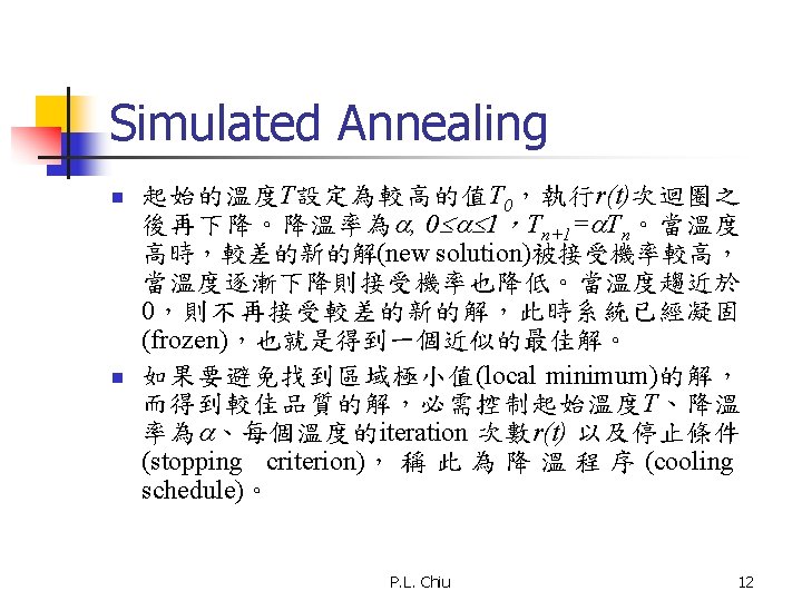
Generic Choices n Kirkpatrick et al. (1983) n n n Set initial value T to be large enough T(t+1)= T(t), : 0. 8~0. 99 N(t): a sufficient number of transitions n n corresponding to thermal equilibrium constant or proportional to the size of the neighborhood Stopping criterion n when the solution obtained at each temperature change is unaltered for a number of consecutive temperature changes. (T…T/10) P. L. Chiu 17

Conclusions n n It is very easy to implement. It can be generally applied to a wide range of problems. SA can provide high quality solutions to many problems. Care is needed to devise an appropriate neighborhood structure and cooling scheduler to obtain an efficient algorithm. P. L. Chiu 18

Outline n n Simulated Annealing Example P. L. Chiu 19

Sensor Placement for Target Location n A complete covered and discriminated sensor field sensor’s coverage 1 2 3 radius=1 4 5 grid point sensor 6 7 8 9 10 11 12 13 14 15 P. L. Chiu 20

Distance Error n n n Due to some resource limitations, a complete discriminated sensor field cannot be constructed. Positioning accuracy, therefore, becomes a major issue of the problem. Distance Error n The distance error of two indistinguishable grid points is defined as the Euclidean distance between them. P. L. Chiu 21

Objectives n Sensor Placement For Target Location n Complete Discrimination n n It is implied that the minimum Hamming distance of power vectors for any pair of grid points will be maximized. High Discrimination n n When complete discrimination is not possible. It is implied that the maximum distance error will be minimized. P. L. Chiu 22

Given Parameters : Index set of the location in the sensor field. : Index set of the sensor’s candidate locations. : Detection radius of sensor located at , : Euclidean distance between location and , : The cost of sensor allocated at location , : Total cost limitation P. L. Chiu 23

Decision Variables : 1, if an sensor is allocated at location , . : A power vector of location , where is 1 if the target at location can be detected by the sensor at location and 0 otherwise. P. L. Chiu 24

Objective Function (K is a big number. ) P. L. Chiu 25

Constraints (1) (2) = (3) (4) 1 (5) P. L. Chiu 26

Constraints (Cont’d) P. L. Chiu 27

The Energy Function n The energy, E, is defined as follows: P. L. Chiu 28

Algorithm 1. Deploy sensors on all grid points // Initial guess 2. repeat until t<tf 3. repeat r times 4. If the cost is still higher than the cost limitation then 5. Discard a sensor randomly 6. Decide the new configuration can be accepted or not 7. If accepted then goto step 10 8. Move a sensor to a new grid point randomly 9. Decide the new configuration can be accepted or not 10. If the best deployment is the desired solution then stop 11. t=t*0. 75, r=r*1. 3 // Cooling function P. L. Chiu 29

Decision for a new deployment // Complete covered P. L. Chiu 30

Energy for the desired solution n The energy for a complete coverage and discrimination deployment is =1 Back to Algorithm P. L. Chiu 31

Parameters n n Initial r 0=5 n, t 0=0. 1 =0. 75, tn+1= tn =1. 3, r(tn+1)= r(tn) tf =1/300 P. L. Chiu 32