G 5 BAIM Artificial Intelligence Methods Graham Kendall

G 5 BAIM Artificial Intelligence Methods Graham Kendall Simulated Annealing

G 5 BAIM Simulated Annealing · Motivated by the physical annealing process · Material is heated and slowly cooled into a uniform structure · Simulated annealing mimics this process · The first SA algorithm was developed in 1953 (Metropolis)

G 5 BAIM Simulated Annealing · Compared to hill climbing the main difference is that SA allows downwards steps · Simulated annealing also differs from hill climbing in that a move is selected at random and then decides whether to accept it · In SA better moves are always accepted. Worse moves are not

G 5 BAIM Simulated Annealing · Kirkpatrick (1982) applied SA to optimisation problems · Kirkpatrick, S , Gelatt, C. D. , Vecchi, M. P. 1983. Optimization by Simulated Annealing. Science, vol 220, No. 4598, pp 671 -680

G 5 BAIM Simulated Annealing The Problem with Hill Climbing · Gets stuck at local minima · Possible solutions · Try several runs, starting at different positions · Increase the size of the neighbourhood (e. g. in TSP try 3 -opt rather than 2 -opt)

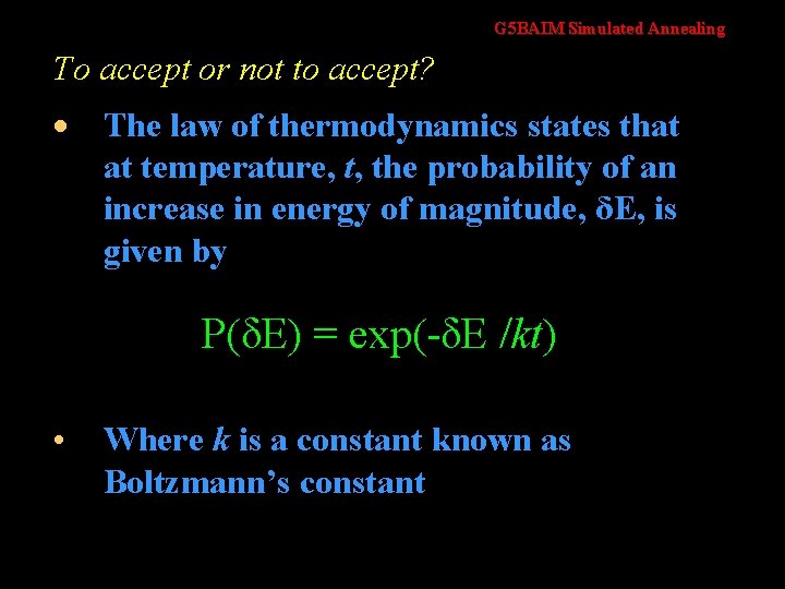
G 5 BAIM Simulated Annealing To accept or not to accept? · The law of thermodynamics states that at temperature, t, the probability of an increase in energy of magnitude, δE, is given by P(δE) = exp(-δE /kt) • Where k is a constant known as Boltzmann’s constant

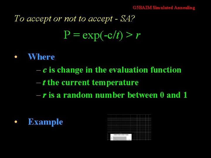
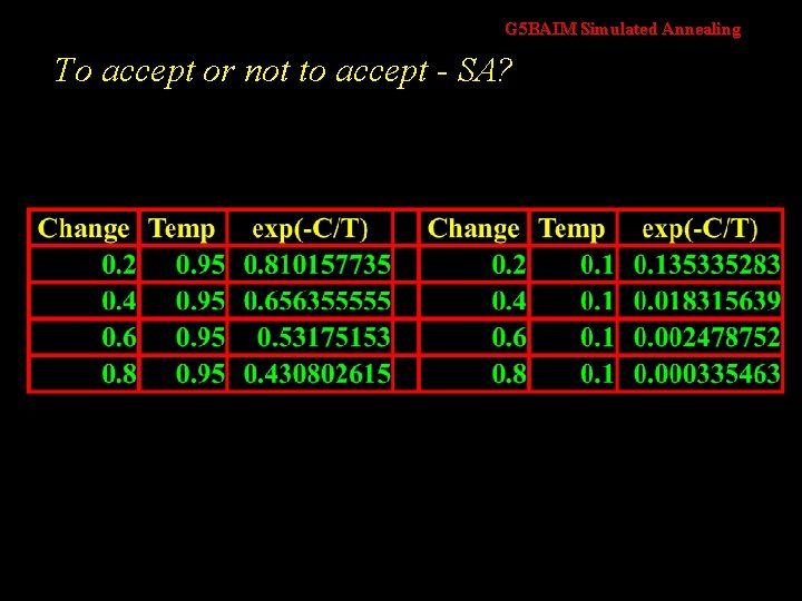
G 5 BAIM Simulated Annealing To accept or not to accept - SA? P = exp(-c/t) > r • Where – c is change in the evaluation function – t the current temperature – r is a random number between 0 and 1 • Example

G 5 BAIM Simulated Annealing To accept or not to accept - SA?

G 5 BAIM Simulated Annealing To accept or not to accept - SA? · The probability of accepting a worse state is a function of both the temperature of the system and the change in the cost function · As the temperature decreases, the probability of accepting worse moves decreases · If t=0, no worse moves are accepted (i. e. hill climbing)

G 5 BAIM Simulated Annealing SA Algorithm · The most common way of implementing an SA algorithm is to implement hill climbing with an accept function and modify it for SA · The example shown here is taken from Russell/Norvig (for consistency with the rest of the course)

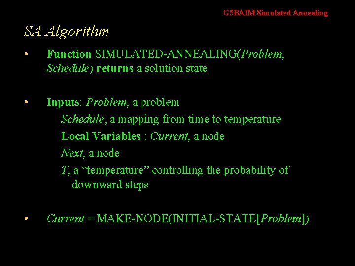
G 5 BAIM Simulated Annealing SA Algorithm • Function SIMULATED-ANNEALING(Problem, Schedule) returns a solution state • Inputs: Problem, a problem Schedule, a mapping from time to temperature Local Variables : Current, a node Next, a node T, a “temperature” controlling the probability of downward steps • Current = MAKE-NODE(INITIAL-STATE[Problem])

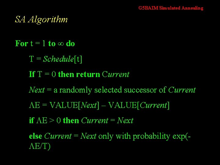
G 5 BAIM Simulated Annealing SA Algorithm For t = 1 to do T = Schedule[t] If T = 0 then return Current Next = a randomly selected successor of Current E = VALUE[Next] – VALUE[Current] if E > 0 then Current = Next else Current = Next only with probability exp( E/T)

G 5 BAIM Simulated Annealing SA Algorithm - Observations • The cooling schedule is hidden in this algorithm - but it is important (more later) • The algorithm assumes that annealing will continue until temperature is zero this is not necessarily the case

G 5 BAIM Simulated Annealing SA Cooling Schedule • Starting Temperature • Final Temperature • Temperature Decrement • Iterations at each temperature

G 5 BAIM Simulated Annealing SA Cooling Schedule - Starting Temperature • Starting Temperature – Must be hot enough to allow moves to almost neighbourhood state (else we are in danger of implementing hill climbing) – Must not be so hot that we conduct a random search for a period of time – Problem is finding a suitable starting temperature

G 5 BAIM Simulated Annealing SA Cooling Schedule - Starting Temperature • Starting Temperature - Choosing – If we know the maximum change in the cost function we can use this to estimate – Start high, reduce quickly until about 60% of worse moves are accepted. Use this as the starting temperature – Heat rapidly until a certain percentage are accepted the start cooling

G 5 BAIM Simulated Annealing SA Cooling Schedule - Final Temperature • Final Temperature - Choosing – It is usual to let the temperature decrease until it reaches zero However, this can make the algorithm run for a lot longer, especially when a geometric cooling schedule is being used – In practise, it is not necessary to let the temperature reach zero because the chances of accepting a worse move are almost the same as the temperature being equal to zero

G 5 BAIM Simulated Annealing SA Cooling Schedule - Final Temperature • Final Temperature - Choosing – Therefore, the stopping criteria can either be a suitably low temperature or when the system is “frozen” at the current temperature (i. e. no better or worse moves are being accepted)

G 5 BAIM Simulated Annealing SA Cooling Schedule - Temperature Decrement • Temperature Decrement – Theory states that we should allow enough iterations at each temperature so that the system stabilises at that temperature – Unfortunately, theory also states that the number of iterations at each temperature to achieve this might be exponential to the problem size

G 5 BAIM Simulated Annealing SA Cooling Schedule - Temperature Decrement • Temperature Decrement – We need to compromise – We can either do this by doing a large number of iterations at a few temperatures, a small number of iterations at many temperatures or a balance between the two

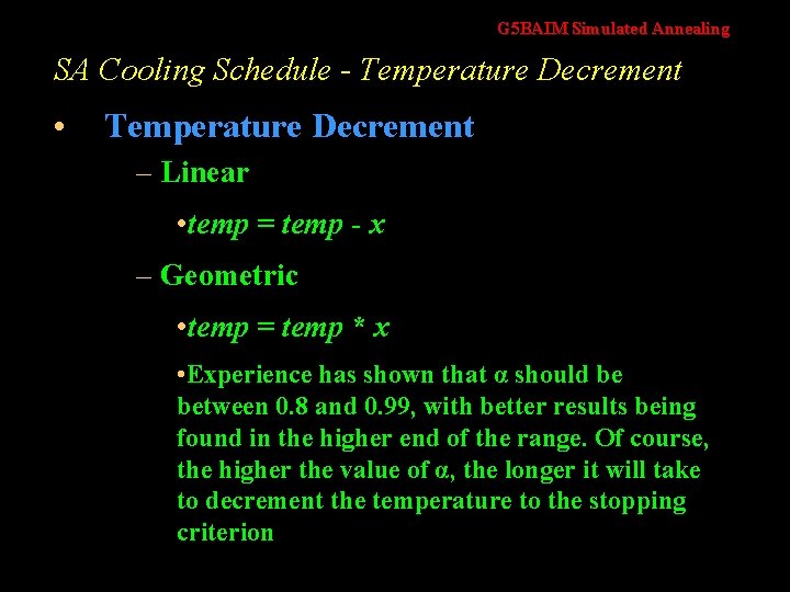
G 5 BAIM Simulated Annealing SA Cooling Schedule - Temperature Decrement • Temperature Decrement – Linear • temp = temp - x – Geometric • temp = temp * x • Experience has shown that α should be between 0. 8 and 0. 99, with better results being found in the higher end of the range. Of course, the higher the value of α, the longer it will take to decrement the temperature to the stopping criterion

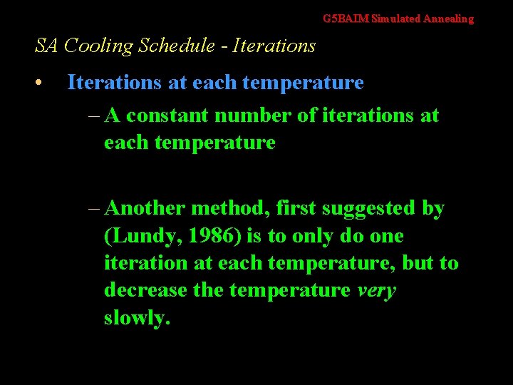
G 5 BAIM Simulated Annealing SA Cooling Schedule - Iterations • Iterations at each temperature – A constant number of iterations at each temperature – Another method, first suggested by (Lundy, 1986) is to only do one iteration at each temperature, but to decrease the temperature very slowly.

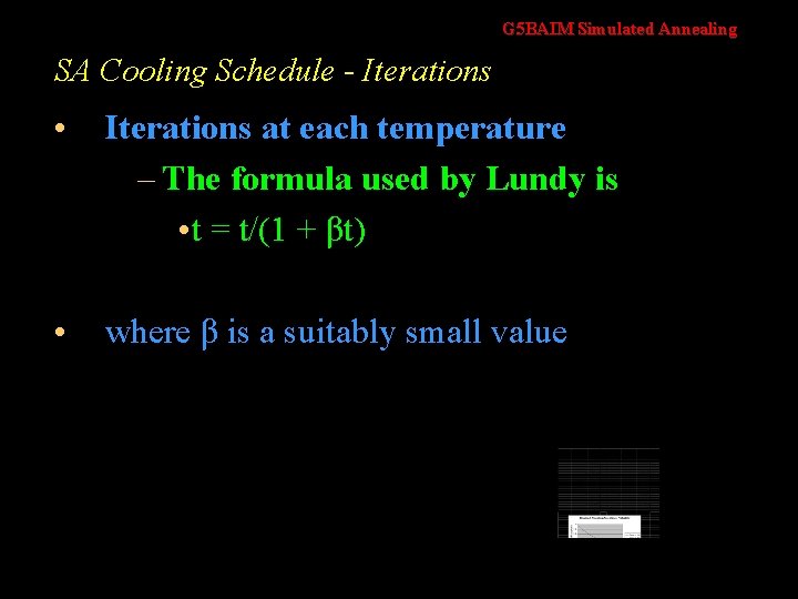
G 5 BAIM Simulated Annealing SA Cooling Schedule - Iterations • Iterations at each temperature – The formula used by Lundy is • t = t/(1 + βt) • where β is a suitably small value

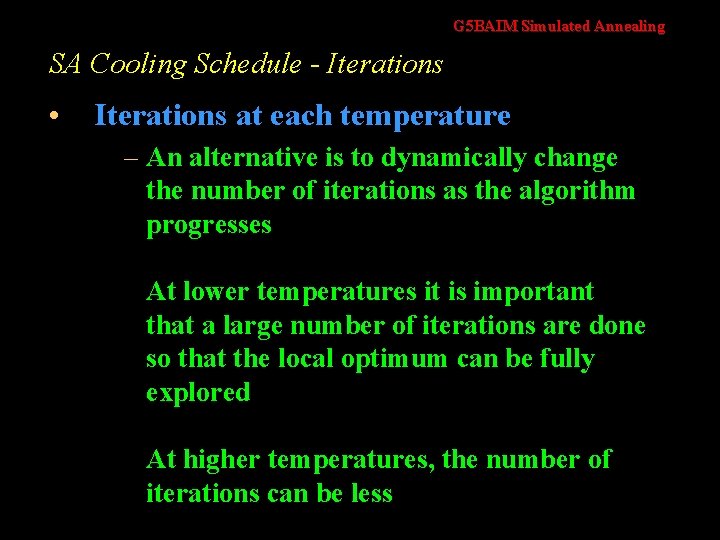
G 5 BAIM Simulated Annealing SA Cooling Schedule - Iterations • Iterations at each temperature – An alternative is to dynamically change the number of iterations as the algorithm progresses At lower temperatures it is important that a large number of iterations are done so that the local optimum can be fully explored At higher temperatures, the number of iterations can be less

G 5 BAIM Simulated Annealing Problem Specific Decisions • The cooling schedule is all about SA but there are other decisions which we need to make about the problem • These decisions are not just related to SA

G 5 BAIM Simulated Annealing Problem Specific Decisions - Cost Function • The evaluation function is calculated at every iteration • Often the cost function is the most expensive part of the algorithm

G 5 BAIM Simulated Annealing Problem Specific Decisions - Cost Function • Therefore – We need to evaluate the cost function as efficiently as possible – Use Delta Evaluation – Use Partial Evaluation

G 5 BAIM Simulated Annealing Problem Specific Decisions - Cost Function • If possible, the cost function should also be designed so that it can lead the search – One way of achieving this is to avoid cost functions where many states return the same value This can be seen as representing a plateau in the search space which the search has no knowledge about which way it should proceed – Bin Packing

G 5 BAIM Simulated Annealing Problem Specific Decisions - Cost Function • Many cost functions cater for the fact that some solutions are illegal. This is typically achieved using constraints – Hard Constraints : these constraints cannot be violated in a feasible solution – Soft Constraints : these constraints should, ideally, not be violated but, if they are, the solution is still feasible

G 5 BAIM Simulated Annealing Problem Specific Decisions - Cost Function • Hard constraints are given a large weighting. The solutions which violate those constraints have a high cost function • Soft constraints are weighted depending on their importance • Weightings can be dynamically changed as the algorithm progresses. This allows hard constraints to be accepted at the start of the algorithm but rejected later

G 5 BAIM Simulated Annealing Problem Specific Decisions - Neighbourhood • How do you move from one state to another? • When you are in a certain state, what other states are reachable?

G 5 BAIM Simulated Annealing Problem Specific Decisions - Neighbourhood • • • Some results have shown that the neighbourhood structure should be symmetric. That is, if you move from state i to state j then it must be possible to move from state j to state i However, a weaker condition can hold in order to ensure convergence. Every state must be reachable from every other. Therefore, it is important, when thinking about your problem to ensure that this condition is met

G 5 BAIM Simulated Annealing Problem Specific Decisions - Performance • What is performance? – Quality of the solution returned – Time taken by the algorithm • We already have the problem of finding suitable SA parameters (cooling schedule)

G 5 BAIM Simulated Annealing Problem Specific Decisions - Performance • Improving Performance - Initialisation – Start with a random solution and let the annealing process improve on that. – Might be better to start with a solution that has been heuristically built (e. g. for the TSP problem, start with a greedy search)

G 5 BAIM Simulated Annealing Problem Specific Decisions - Performance • Improving Performance - Hybridisation – or memetic algorithms – Combine two search algorithms – Relatively new research area

G 5 BAIM Simulated Annealing Problem Specific Decisions - Performance • Improving Performance - Hybridisation – Often a population based search strategy is used as the primary search mechanism and a local search mechanism is applied to move each individual to a local optimum – It may be possible to apply some heuristic to a solution in order to improve it

G 5 BAIM Simulated Annealing SA Modifications - Acceptance Probability • The probability of accepting a worse move is normally based on the physical analogy (based on the Boltzmann distribution) • But is there any reason why a different function will not perform better for all, or at least certain, problems?

G 5 BAIM Simulated Annealing SA Modifications - Acceptance Probability • Why should we use a different acceptance criteria? – The one proposed does not work. Or we suspect we might be able to produce better solutions – The exponential calculation is computationally expensive. – (Johnson, 1991) found that the acceptance calculation took about one third of the computation time

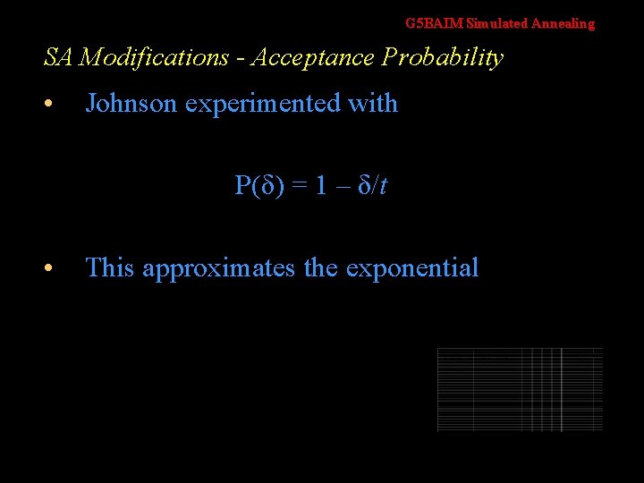
G 5 BAIM Simulated Annealing SA Modifications - Acceptance Probability • Johnson experimented with P(δ) = 1 – δ/t • This approximates the exponential

G 5 BAIM Simulated Annealing SA Modifications - Acceptance Probability • • • A better approach was found by building a look-up table of a set of values over the range δ/t During the course of the algorithm δ/t was rounded to the nearest integer and this value was used to access the look-up table This method was found to speed up the algorithm by about a third with no significant effect on solution quality

G 5 BAIM Simulated Annealing SA Modifications - Cooling • If you plot a typical cooling schedule you are likely to find that at high temperatures many solutions are accepted • If you start at too high a temperature a random search is emulated and until the temperature cools sufficiently any solution can be reached and could have been used as a starting position

G 5 BAIM Simulated Annealing SA Modifications - Cooling • At lower temperatures, a plot of the cooling schedule, is likely to show that very few worse moves are accepted; almost making simulated annealing emulate hill climbing

G 5 BAIM Simulated Annealing SA Modifications - Cooling • Taking this one stage further, we can say that simulated annealing does most of its work during the middle stages of the cooling schedule • (Connolly, 1990) suggested annealing at a constant temperature

G 5 BAIM Simulated Annealing SA Modifications - Cooling • But what temperature? • It must be high enough to allow movement but not so low that the system is frozen • But, the optimum temperature will vary from one type of problem to another and also from one instance of a problem to another instance of the same problem

G 5 BAIM Simulated Annealing SA Modifications - Cooling • • One solution to this problem is to spend some time searching for the optimum temperature and than stay at that temperature for the remainder of the algorithm The final temperature is chosen as the temperature that returns the best cost function during the search phase

G 5 BAIM Simulated Annealing SA Modifications - Neighbourhood • • • The neighbourhood of any move is normally the same throughout the algorithm but… The neighbourhood could be changed as the algorithm progresses For example, a cost function based on penalty values can be used to restrict the neighbourhood if the weights associated with the penalties are adjusted as the algorithm progresses

G 5 BAIM Simulated Annealing SA Modifications - Cost Function • The cost function is calculated at every iteration of the algorithm • Various researchers (e. g. Burke, 1999) have shown that the cost function can be responsible for a large proportion of the execution time of the algorithm • Some techniques have been suggested which aim to alleviate this problem

G 5 BAIM Simulated Annealing SA Modifications - Cost Function • (Rana, 1996) - Coors Brewery – GA but could be applied to SA – The evaluation function is approximated (one tenth of a second) – Potentially good solution are fully evaluated (three minutes)

G 5 BAIM Simulated Annealing SA Modifications - Cost Function • (Ross, 1994) uses delta evaluation on the timetabling problem – Instead of evaluating every timetable as only small changes are being made between one timetable and the next, it is possible to evaluate just the changes and update the previous cost function using the result of that calculation

G 5 BAIM Simulated Annealing SA Modifications - Cost Function • (Burke, 1999) uses a cache – The cache stores cost functions (partial and complete) that have already been evaluated – They can be retrieved from the cache rather than having to go through the evaluation function again

G 5 BAIM Artificial Intelligence Methods Graham Kendall End of Simulated Annealing