Simulated Annealing The Basics and Pseudo Code SA

Simulated Annealing The Basics and Pseudo Code

SA Basics • Fundamentally simple algorithm – Not much more intelligent than guessing • Relies on the algorithm’s ability to span the search space effectively • Uses simple but effective means to avoid local minima • Name derives from a technique in metallurgy where two metals are fused by melting them and slowly cooling the combination

SA Glossary • Solution: An answer to a problem without respect to its apparent “value” • Neighbor: A solution which is “next” to a given solution in the solution space (or neighborhood) • Fitness: The “value” of a solution • Temperature: The current average rate at which less fit solutions are accepted • Annealing Schedule: The function which lowers (or raises) the temperature the algorithm uses during its search

SA Pseudo Code S 0 = Generate. Solution() Temp = START_TEMP K = 0 // iteration count while(!stopping_condition(S 0, Temp, K)) S 1 = Neighbor(S 0) // make a neighbor of S 0 if(Fitness(S 1) < Fitness(S 0)) S 0 = S 1 // if S 1 is better than S 0 take it else if(rand() < temp. Func(S 0, S 1, Temp, K)) S 0 = S 1 // if S 1 is worse than S 0 // conditionally take it end if Annealing. Schedule(S 0, Temp, K) // anneal the temp K = K + 1 // increase the iteration count end while

What is a Neighbor? • A neighbor is just a permutation based on the current solution • This is how the algorithm moves around the search space • In the fuel bundle given to the right a neighbor would be a different arrangement of the fuel pins

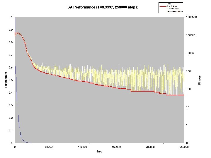
Why Temperature? • Simulated Annealing uses temperature as a way to leave local minima • Hill climbing can get stuck – Unable to move outside the minima as it does not take worse neighbors • SA uses an annealing schedule to determine how high the temperature should be, and how long it should remain at a given temperature

What Annealing Schedule? • This is a complicated question! – There are linear schedules, geometric schedules, oscillating schedules, schedules based on the rate of improvement – Some SA algorithms use a GA to design their annealing schedule! • A very basic, yet effective, annealing schedule is one that is geometric, but stepped – T = T * 0. 9996 – However, this is only done every M iterations, which is either determined by the rate of improvement or by a hard figure (say every 1000 iterations) – Quantitative analysis is the only way to determine the most effective schedule

Putting it all Together • When the new solution is found to be worse than the old solution you must evaluate if the bad solution should be taken • Another choice must be made! How do you interpret the temperature? • The Metropolis-Hastings algorithm is commonly used (and has interesting ties to SA) – The algorithm approximates a probability distribution and was created specifically for the Boltzmann Distribution – The algorithm allows you to create samples for problems where it is hard to effectively sample the entire space • This sounds exactly like what SA requires!

Metropolis-Hastings • e(-(Fitness(S 1) – Fitness(S 0)) / (K * Temp)) • This method was given by Kirkpatrick et. al and doesn’t exactly replicate what occurs in natural annealing • Based on the relative difference in how bad the new solution is and how far along the algorithm is running, the Metropolis-Hastings approach takes bad guesses frequently while the temperature is high, and eventually settles into a descent until a minima is found

Conclusion • Simple changes to a greedy or hill climbing algorithm can make effective use of computational resources to find solutions in a solution space too hard or large to sample fully • Simulated Annealing can be applied to many applications due to extremely simple nature • Simulated Annealing can be a good choice for a first guess solution to optimizing a problem – For certain problems, SA is among the best solutions for finding optimal answers to a problem