SIMPOSIO Gli eventi estremi alla ricerca di un

SIMPOSIO “Gli eventi estremi: alla ricerca di un paradigma scientifico” Alghero, 24 -26 Settembre 2003 Probabilistic modelling of drought characteristics G. Rossi, B. Bonaccorso, A. Cancelliere Department of Civil and Environmental Engineering University of Catania

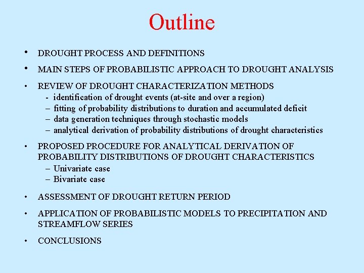
Outline • DROUGHT PROCESS AND DEFINITIONS • MAIN STEPS OF PROBABILISTIC APPROACH TO DROUGHT ANALYSIS • REVIEW OF DROUGHT CHARACTERIZATION METHODS - identification of drought events (at-site and over a region) – fitting of probability distributions to duration and accumulated deficit – data generation techniques through stochastic models – analytical derivation of probability distributions of drought characteristics • PROPOSED PROCEDURE FOR ANALYTICAL DERIVATION OF PROBABILITY DISTRIBUTIONS OF DROUGHT CHARACTERISTICS – Univariate case – Bivariate case • ASSESSMENT OF DROUGHT RETURN PERIOD • APPLICATION OF PROBABILISTIC MODELS TO PRECIPITATION AND STREAMFLOW SERIES • CONCLUSIONS

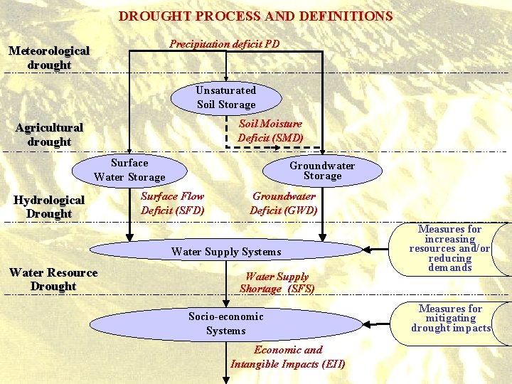
DROUGHT PROCESS AND DEFINITIONS Precipitation deficit PD Meteorological drought Unsaturated Soil Storage Soil Moisture Deficit (SMD) Agricultural drought Surface Water Storage Hydrological Drought Groundwater Storage Surface Flow Deficit (SFD) Groundwater Deficit (GWD) Water Supply Systems Water Resource Drought Water Supply Shortage (SFS) Socio-economic Systems Economic and Intangible Impacts (EII) Measures for increasing resources and/or reducing demands Measures for mitigating drought impacts

DROUGHT DEFINITIONS (1/2) Meteorological drought : precipitation deficit (drought input) caused by atmospheric fluctuations related to: i) solar energy fluctuations (? ) ii) earth processes (geophysical oceanographic interactions) iii) biosphere feedbacks Agricultural drought : soil moisture deficit deriving from meteorological drought routed trough soil storage mechanism (time delay and amount change)

DROUGHT DEFINITIONS (2/2) Hydrological drought : surface flow deficit and groundwater deficit deriving respectively from precipitation deficit and soil moisture deficit routed trough the storage mechanism in natural water bodies Water Resources drought : water supply shortage (drought output) influenced by artificial storage features (reservoir capacity and operation rules) and by different drought mitigation measures

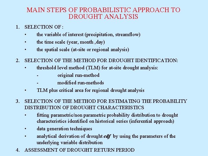
MAIN STEPS OF PROBABILISTIC APPROACH TO DROUGHT ANALYSIS 1. SELECTION OF : • the variable of interest (precipitation, streamflow) • the time scale (year, month , day) • the spatial scale (at-site or regional analysis) 2. SELECTION OF THE METHOD FOR DROUGHT IDENTIFICATION: • threshold level method (TLM) for at-site drought analysis: original run-method modified run-methods • TLM plus critical area for regional drought analysis 3. SELECTION OF THE METHOD FOR ESTIMATING THE PROBABILITY DISTRIBUTION OF DROUGHT CHARACTERISTICS • fitting parametric/non parametric probability distribution to drought characteristics identified on historical series (inferential approach) • data generation techniques • analytical derivation of drought cdf by using the parameters of the underlying variable distribution 4. ASSESSMENT OF DROUGHT RETURN PERIOD

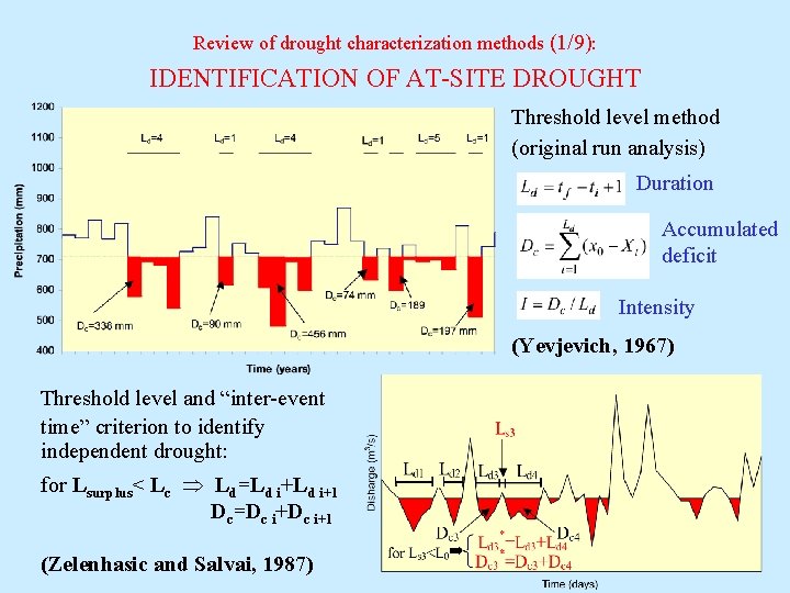
Review of drought characterization methods (1/9): IDENTIFICATION OF AT-SITE DROUGHT Threshold level method (original run analysis) Duration Accumulated deficit Intensity (Yevjevich, 1967) Threshold level and “inter-event time” criterion to identify independent drought: for Lsurplus< Lc Ld=Ld i+1 Dc=Dc i+1 (Zelenhasic and Salvai, 1987)

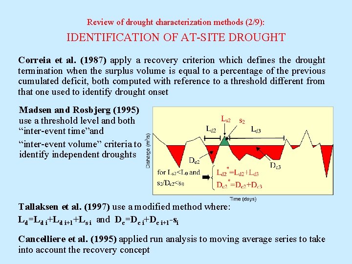
Review of drought characterization methods (2/9): IDENTIFICATION OF AT-SITE DROUGHT Correia et al. (1987) apply a recovery criterion which defines the drought termination when the surplus volume is equal to a percentage of the previous cumulated deficit, both computed with reference to a threshold different from that one used to identify drought onset Madsen and Rosbjerg (1995) use a threshold level and both “inter-event time”and “inter-event volume” criteria to identify independent droughts Tallaksen et al. (1997) use a modified method where: Ld=Ld i+1+Ls i and Dc=Dc i+1 -si Cancelliere et al. (1995) applied run analysis to moving average series to take into account the recovery concept

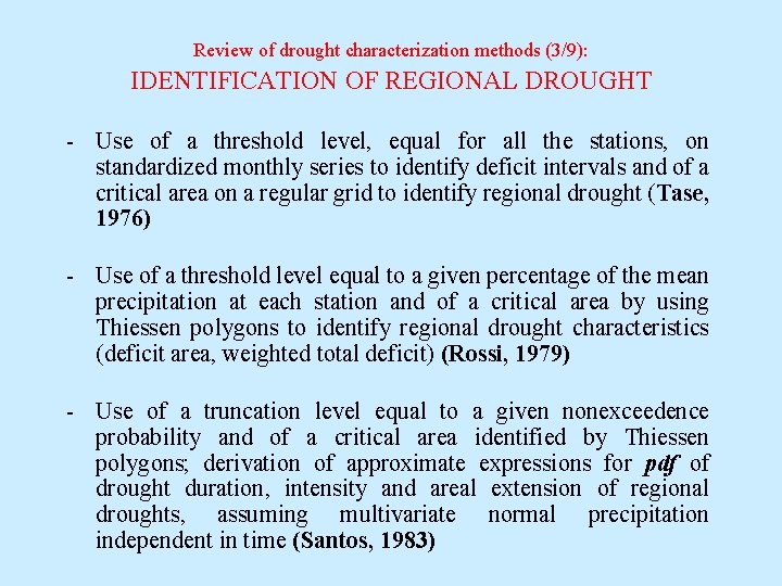
Review of drought characterization methods (3/9): IDENTIFICATION OF REGIONAL DROUGHT - Use of a threshold level, equal for all the stations, on standardized monthly series to identify deficit intervals and of a critical area on a regular grid to identify regional drought (Tase, 1976) - Use of a threshold level equal to a given percentage of the mean precipitation at each station and of a critical area by using Thiessen polygons to identify regional drought characteristics (deficit area, weighted total deficit) (Rossi, 1979) - Use of a truncation level equal to a given nonexceedence probability and of a critical area identified by Thiessen polygons; derivation of approximate expressions for pdf of drought duration, intensity and areal extension of regional droughts, assuming multivariate normal precipitation independent in time (Santos, 1983)

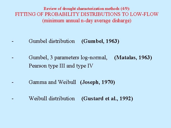
Review of drought characterization methods (4/9): FITTING OF PROBABILITY DISTRIBUTIONS TO LOW-FLOW (minimum annual n-day average disharge) - Gumbel distribution - Gumbel, 3 parameters log-normal, Pearson type III and type IV - Gamma and Weibull (Joseph, 1970) - Weibull distribution (Gumbel, 1963) (Matalas, 1963) (Gustard et al. , 1992)

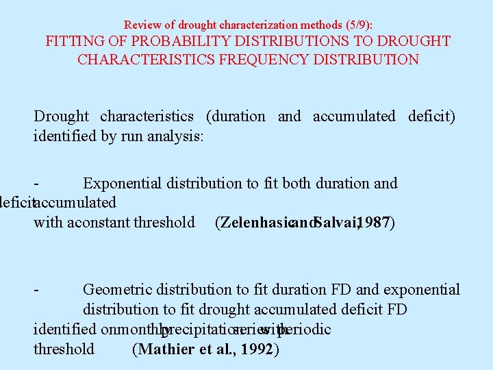
Review of drought characterization methods (5/9): FITTING OF PROBABILITY DISTRIBUTIONS TO DROUGHT CHARACTERISTICS FREQUENCY DISTRIBUTION Drought characteristics (duration and accumulated deficit) identified by run analysis: Exponential distribution to fit both duration and deficitaccumulated with a constant threshold (Zelenhasicand. Salvai, 1987) - Geometric distribution to fit duration FD and exponential distribution to fit drought accumulated deficit FD identified onmonthly precipitation series with periodic threshold (Mathier et al. , 1992)

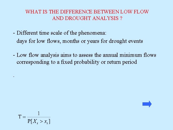
WHAT IS THE DIFFERENCE BETWEEN LOW FLOW AND DROUGHT ANALYSIS ? - Different time scale of the phenomena: days for low flows, months or years for drought events - Low flow analysis aims to assess the annual minimum flows corresponding to a fixed probability or return period -

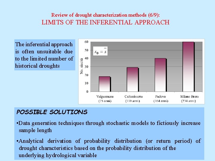
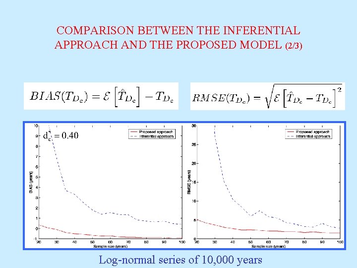
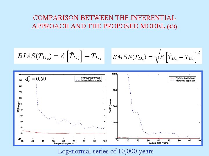
Review of drought characterization methods (6/9): LIMITS OF THE INFERENTIAL APPROACH The inferential approach is often unsuitable due to the limited number of historical droughts POSSIBLE SOLUTIONS • Data generation techniques through stochastic models to fictiously increase sample length • Analytical derivation of probability distribution (or return period) of drought characteristics based on the probability distribution of the underlying hydrological variable

Review of drought characterization methods (7/9): DATA GENERATION TECHNIQUES - Log-normal distribution to fit FD of the longest negative run length and the largest run sum obtained by lag-one autoregressive generated samples (Millan and Yevjevich, 1971) - Negative Binomial distribution to fit FD of run length and Pearson distribution to fit FD of run sum obtained by a bivariate lag-one autoregressive model (Guerrero and Yevjevich, 1975) - Beta distribution to fit the FD of regional drought characteristics (deficit area, areal deficit and intensity) obtained by generating monthly precipitation series (time independent but space dependent variable) (Tase, 1976 ) - Gamma distribution to fit the conditional distribution of drought accumulated deficit given drought duration (Shiau and Shen, 2001)

Review of drought characterization methods (8/9): ANALYTICAL DERIVATION OF DROUGHT CHARACTERISTICS PROBABILITY DISTRIBUTION 1967 Downer et al. (distribution and moments of run-length and run-sum derived for i. i. d. random variables) 1969 Llamas and Siddiqui (distribution function and moments of run-length, run-sum and run -intensity derived for independent normal and gamma series) 1970 Saldarriaga and Yevjevich (exact and approximate expressions of probabilities of run of wet and dry years for either independent or dependent stationary series of variables following the 1 st order linear autoregressive model) 1976 Sen (probability of run-length for stationary lag-1 Markov process) 1977 Sen (moments of run-sum for independent and two-state Markov process) 1980 Sen (distribution of max deficit for stationary Markov process)

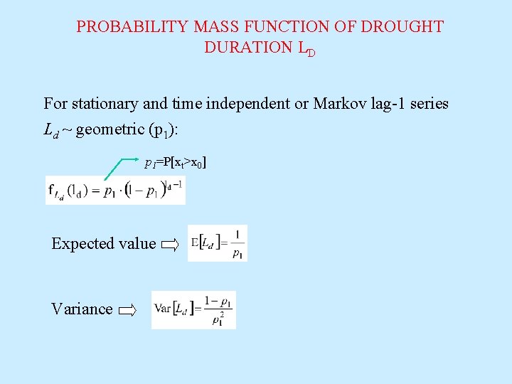
PROBABILITY MASS FUNCTION OF DROUGHT DURATION LD For stationary and time independent or Markov lag-1 series Ld ~ geometric (p 1): p 1=P[xt>x 0] Expected value Variance

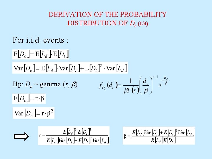
DERIVATION OF THE PROBABILITY DISTRIBUTION OF Dc (1/4) For i. i. d. events : Hp: Dc ~ gamma (r, b)

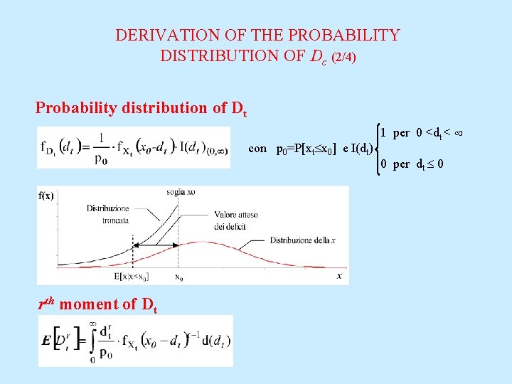
DERIVATION OF THE PROBABILITY DISTRIBUTION OF Dc (2/4) Probability distribution of Dt con p 0=P[xt x 0] e I(dt) rth moment of Dt 1 per 0 <dt < 0 per dt 0

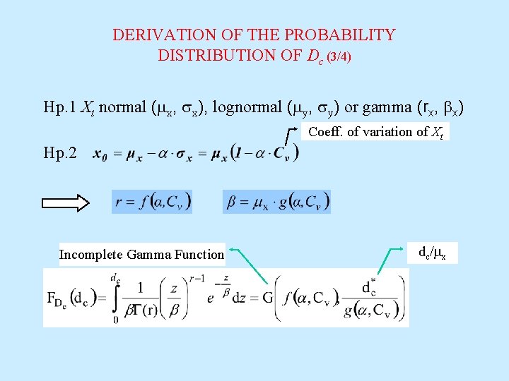
DERIVATION OF THE PROBABILITY DISTRIBUTION OF Dc (3/4) Hp. 1 Xt normal (mx, sx), lognormal (my, sy) or gamma (rx, bx) Coeff. of variation of Xt Hp. 2 Incomplete Gamma Function dc/mx

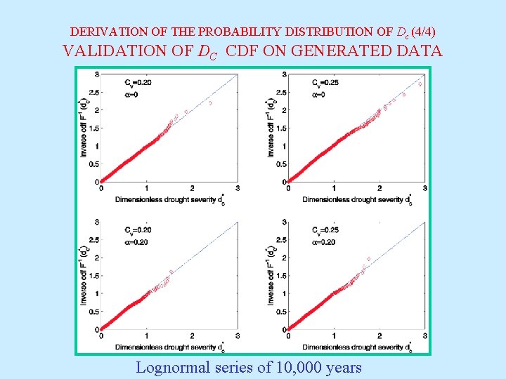
DERIVATION OF THE PROBABILITY DISTRIBUTION OF Dc (4/4) VALIDATION OF DC CDF ON GENERATED DATA Lognormal series of 10, 000 years

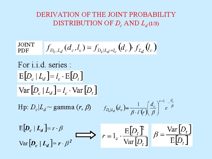
DERIVATION OF THE JOINT PROBABILITY DISTRIBUTION OF Dc AND Ld (1/3) JOINT PDF For i. i. d. series : Hp: Dc|Ld ~ gamma (r, b)

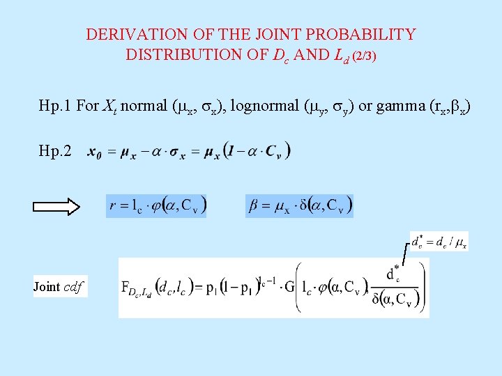
DERIVATION OF THE JOINT PROBABILITY DISTRIBUTION OF Dc AND Ld (2/3) Hp. 1 For Xt normal (mx, sx), lognormal (my, sy) or gamma (rx, bx) Hp. 2 Joint cdf

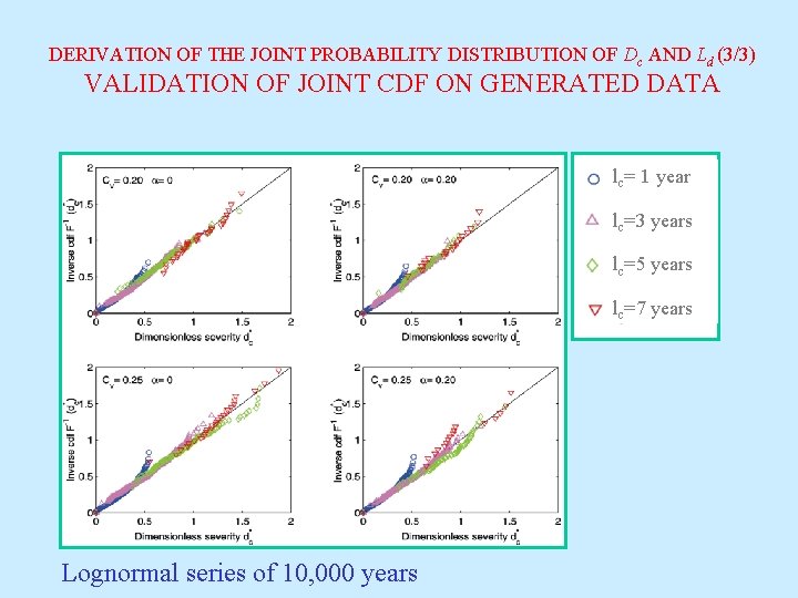
DERIVATION OF THE JOINT PROBABILITY DISTRIBUTION OF Dc AND Ld (3/3) VALIDATION OF JOINT CDF ON GENERATED DATA lc= 1 year lc=3 years lc=5 years lc=7 years Lognormal series of 10, 000 years

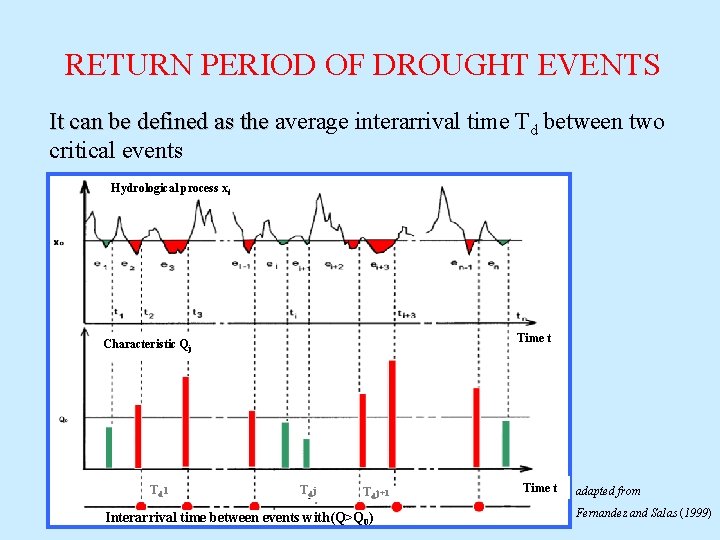
RETURN PERIOD OF DROUGHT EVENTS It can be defined as the average interarrival time Td between two critical events Hydrological process xt Time t Characteristic Qj Td 1 Td j+1 Interarrival time between events with(Q>Q 0) Time t adapted from Fernandez and Salas (1999)

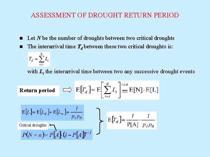
ASSESSMENT OF DROUGHT RETURN PERIOD n n Let N be the number of droughts between two critical droughts The interarrival time Td between these two critical droughts is: with Li the interarrival time between two any successive drought events Return period Critical droughts

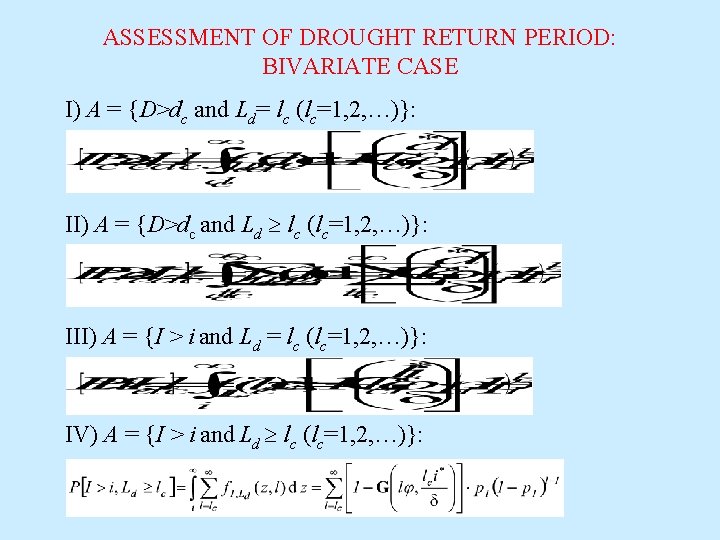
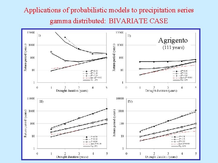
ASSESSMENT OF DROUGHT RETURN PERIOD: BIVARIATE CASE I) A = {D>dc and Ld= lc (lc=1, 2, …)}: II) A = {D>dc and Ld lc (lc=1, 2, …)}: III) A = {I > i and Ld = lc (lc=1, 2, …)}: IV) A = {I > i and Ld lc (lc=1, 2, …)}:

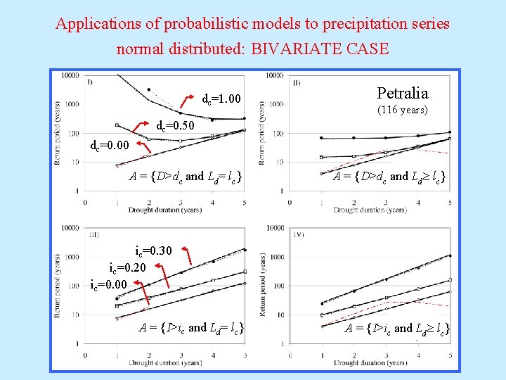
Applications of probabilistic models to precipitation series normal distributed: BIVARIATE CASE dc=1. 00 Petralia (116 years) dc=0. 50 dc=0. 00 A = {D>dc and Ld= lc} A = {D>dc and Ld lc} ic=0. 30 ic=0. 20 ic=0. 00 A = {I>ic and Ld= lc} A = {I>ic and Ld lc}

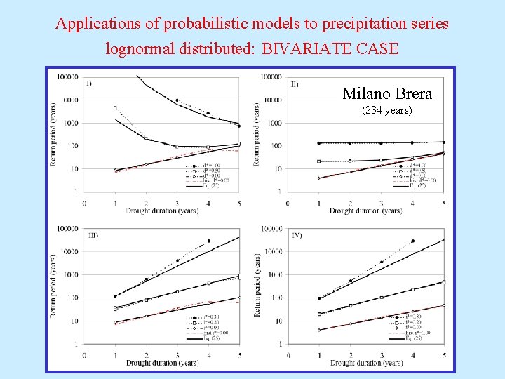
Applications of probabilistic models to precipitation series lognormal distributed: BIVARIATE CASE Milano Brera (234 years)

Applications of probabilistic models to precipitation series gamma distributed: BIVARIATE CASE Agrigento (111 years)

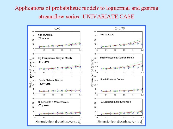
Applications of probabilistic models to lognormal and gamma streamflow series: UNIVARIATE CASE (82 years) (51 years) (100 years) (53 years)

Applications of probabilistic models to lognormal and gamma streamflow series: BIVARIATE CASE (82 years) (51 years) (100 years) (53 years)

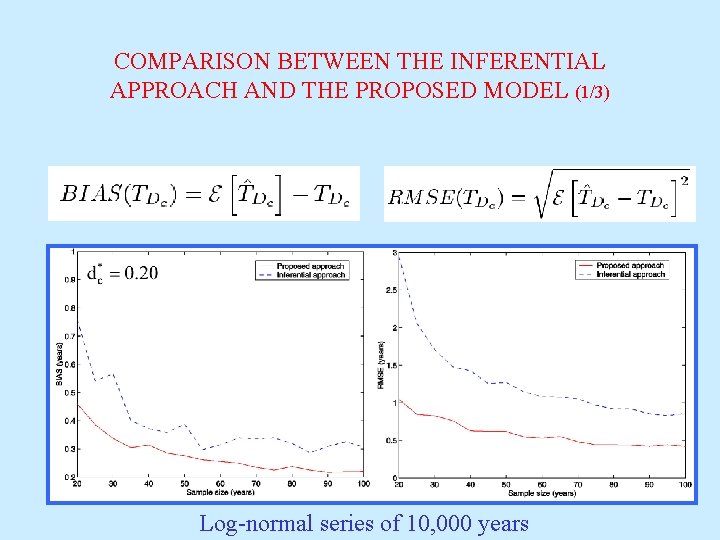
COMPARISON BETWEEN THE INFERENTIAL APPROACH AND THE PROPOSED MODEL (1/3) Log-normal series of 10, 000 years

COMPARISON BETWEEN THE INFERENTIAL APPROACH AND THE PROPOSED MODEL (2/3) Log-normal series of 10, 000 years

COMPARISON BETWEEN THE INFERENTIAL APPROACH AND THE PROPOSED MODEL (3/3) Log-normal series of 10, 000 years

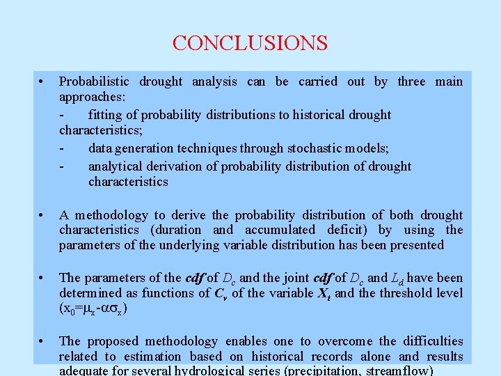
CONCLUSIONS • Probabilistic drought analysis can be carried out by three main approaches: fitting of probability distributions to historical drought characteristics; data generation techniques through stochastic models; analytical derivation of probability distribution of drought characteristics • A methodology to derive the probability distribution of both drought characteristics (duration and accumulated deficit) by using the parameters of the underlying variable distribution has been presented • The parameters of the cdf of Dc and the joint cdf of Dc and Ld have been determined as functions of Cv of the variable Xt and the threshold level (x 0=mx-asx) • The proposed methodology enables one to overcome the difficulties related to estimation based on historical records alone and results adequate for several hydrological series (precipitation, streamflow)