Shrinkage Methods for Variable Selection Statisticians like artists

Shrinkage Methods for Variable Selection “Statisticians, like artists, have the bad habit of falling in love with their models. ” -George Box

Ordinary Least Squares • Linear Model: Minimize Sum of Squares due to Errors

Limitations • Decompose error into bias and variance term, linear regression focuses on bias and suffers from high variance. Bias variance trade-off. • Unstable, variance inflation with large number of predictors, specially correlated predictors. • Inverting becomes problematic.
 • Very much like least squares but minimizes")
Ridge Regression (Hoerl and Kennard, 1988) • Very much like least squares but minimizes a loss function + penalty term • Adding to the diagonals of the matrix to make inversion possible. • Shrinks coefficients to zero

N=50, p=30, 10 large and 20 small coefficients http: //www. stat. cmu. edu/~ryantibs/datamining/lectures

Tuning Parameter • Here is a tuning parameter which controls how much you penalize. • When is zero, you get back linear regression. • When what happens? • In between values of does the balancing act. Bias increases and variance decreases as increases. • You will center and scale the predictors before doing ridge regression

Optimal amount of shrinkage http: //www. stat. cmu. edu/~ryantibs/datamining/lectures

How to choose the tuning parameter? • This is actually a hard question • Golub et al (1979) proposed to use generalized cross-validation to select • GCV is a weighted modification of ordinary leave 1 out cross validation (like PRESS) • It has certain asymptotic optimality properties (Craven and Wahba, 1979) • In R: library(MASS) function lm. ridge • Or look at library(glmnet)

Ubiquitous and Daunting

Variable Selection • Suppose there is a group of variables where the true coefficient is really zero. • Identifying relevant predictors from a larger set is defined as variable selection • Ridge does not perform variable selection • In the case when some coefficients are truly zero, ridge can still outperform linear regression for a narrower range of • You really wanted to identify a subset…
")
A landmark paper (1996)

Shrinking coefficients to zero • Instead of the sum of squares of betas or the L 2 norm, use L 1 norm in the penalty • LASSO: Least absolute shrinkage and selection operator.

Tuning Parameter • Here is a tuning parameter which controls how much you penalize. • When is zero, you get back linear regression. • When what happens? • In between values of does the balancing act. Bias increases and variance decreases as increases. Some betas shrunk to zero. • You will center and scale the predictors before doing LASSO

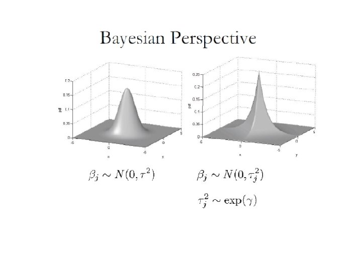
Why LASSO shrinks coefficients to zero and can perform variable selection You can touch the contour ellipse for the first time at a corner of the square, corresponding to a zero coefficient. In ridge there are no corners for the contour to hit, zero solutions will rarely result.

Ridge versus LASSO in a sample dataset: note Coefficients go to zero as increases.
 set. seed(0)# set up the randomnumber-generator seed for cross validation (CV)")
R implementation library('gcdnet') set. seed(0)# set up the randomnumber-generator seed for cross validation (CV) cv. lasso<cv. gcdnet(x, y, lambda 2=0, method="l s")#The default is 5 -fold CV plot(cv. lasso) # the CV error plot
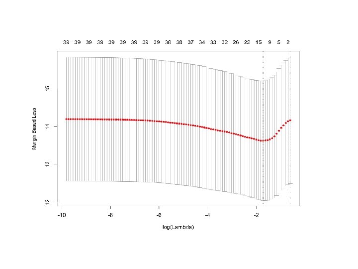

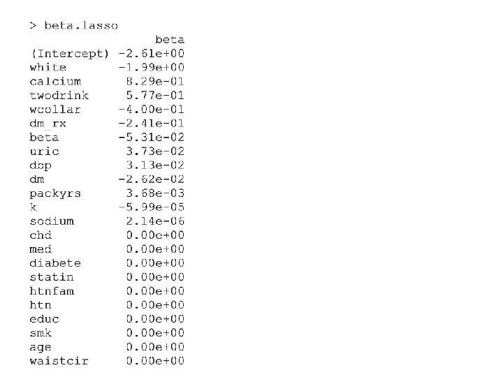
Choosing optimal lambda by CV cv. lasso$lambda #the values of the candidate lambda log(cv. lasso$lambda)#the values of log(lambda) lambda. opt=cv. lasso$lambda. min#value of lambda that gives minimum mean cross-validated error lambda. opt [1] 0. 178 Implement LASSO with this chosen optimal value fit. lasso=gcdnet(x, y, lambda=lambda. opt, lambda 2=0, method="ls") beta. lasso=coef(fit. lasso)# get the coefficients #beta. lasso order=order(abs(beta. lasso), decreasing = TRUE)# sorted by absolute value of beta in decreasing order beta. lasso=data. frame(beta=beta. lasso[order], row. names=rowname s(beta. lasso)[order]) beta. lasso
 • LASSO does not do very well for")
Elastic Net (Zou and Hastie, 2005) • LASSO does not do very well for a correlated set of predictors and when p much larger than n. • If there is a group of predictors with high pairwise correlation, LASSO tends to select only one from the group and does not care which one it is. • Prediction performance of LASSO not satisfactory with highly correlated set of predictors, dominated by ridge.

Modify LASSO to fix this LASSO and Ridge Regression are special cases

Elastic Net Combining L 1 and L 2 penalties R package GLMNET GCDNET SAS GLMSELECT (only linear models)

LASSO vs ENET • ENET beats LASSO in presence of collinearity in terms of prediction error • Produces larger models than LASSO • Produces sparse models with good prediction accuracy while encouraging grouping effect.
#the number of observations; set. seed(0) # set up a seed")
R implementation num. obs=nrow(x)#the number of observations; set. seed(0) # set up a seed for the random number generator "sample“ foldid=sample(rep(seq(5), length=num. obs))# this is to make sure lambda 2 is cross-validated by the same training/validation sets # 5 means we do 5 -fold cross validation which is default in gcdnet
 #candidate lambda 2")
Choose lambda 2 first lambda 2. list=seq(0. 01, 2, by=0. 01) #candidate lambda 2 num. lambda 2=length(lambda 2. list) #the number of candidate lambda 2 min. cv=numeric(num. lambda 2)
 {cv.")
#cross validation for each candidate lambda 2 for(i in 1: num. lambda 2) {cv. enet=cv. gcdnet(x, y, foldid=fold id, lambda 2=lambda 2. list[i], method= "ls") # lambda (for L 1 penalty) will be automatically generated by default setting min. cv[i]=min(cv. enet$cvm) #collect minimum cv error for each lambda 2 candidate}

plot(lambda 2. list, min. cv, xlab="la mbda 2", ylab="minimum CV error", main="minimum CV error given lambda 2", type='l')
![lambda 2. opt=lambda 2. list[which. mi n(min. cv)] #optimal lambda 2 that has the](http://slidetodoc.com/presentation_image_h2/e4df697eb7618475cb86bedac64e71f5/image-29.jpg "lambda 2. opt=lambda 2. list[which. mi n(min. cv)] #optimal lambda 2 that has the")
lambda 2. opt=lambda 2. list[which. mi n(min. cv)] #optimal lambda 2 that has the minimum CV error lambda 1. list=cv. enet$lambda #candidate lambda (for L 1 penalty) #cross validation for lambda 1 given the optimal lambda 2 cv. enet=cv. gcdnet(x, y, foldid=fold id, lambda 2=lambda 2. opt, method="ls ") plot(cv. enet) #CV error given lambda 1 and the optimal lambda 2
 #CV error given lambda 1 and the optimal lambda 2")
plot(cv. enet) #CV error given lambda 1 and the optimal lambda 2
 fit. enet=gcdnet(x, y, lambda=exp(1. 5), lambda 2=lambda 2. opt, method=\" ls\")")
#try lambda=exp(-1. 5) fit. enet=gcdnet(x, y, lambda=exp(1. 5), lambda 2=lambda 2. opt, method=" ls") beta. enet=coef(fit. enet)# get the coefficients order=order(abs(beta. enet), decrea sing = TRUE)# sorted by absolute value of beta in decreasing order beta. enet=data. frame(beta=beta. en et[order], row. names=rownames(beta. enet)[order])

Sample coefficient vector

Adaptive LASSO and ENET • We have just been getting beta vectors • What about CI for beta? P-value for testing? • Often people will choose variables with non-zero coefficients and go back to run the usual linear model. Incorrect! • Inference post model selection is hard!
 • Use a weighted L 1 penalty. • An asymptotic")
Zou and Zhang (2009) • Use a weighted L 1 penalty. • An asymptotic result that produces standard error and p-values for each nonzero estimated coefficient. • Adaptive LASSO is a special case of adaptive ENET by forcing lambda 2=0.

Math and more math: useful

Adaptive ENET We choose the initial estimates by regular ENET R codes for getting Adaptive ENET and Adaptive LASSO p-values and std errors are complicated and are provided in the R code folder

After a chain of complex R codes Adaptive LASSO inference

Comparing with OLS on selected predictors Note much larger P-values for the last two predictors using Adaptive LASSO inference rather than running linear model for predictors with non-zero coefficients

Adaptive ENET on same data Adaptive ENET inference

Comparison with OLS Note much larger P-values for the last two predictors using Adaptive ENET inference rather than running linear model for predictors with non-zero coefficients

Moral of the story • You just went through a very dense lecture • Regularized variable selection with penalty terms is a new area of research where a lot of the things including how to do post model selection inference are still evolving. • These are very useful tools when there truly exists a small subset of important predictors (sparsity).
- Slides: 41