session the perfectly competitive market four the monopolist

session the perfectly competitive market four the monopolist problem …………. 1 the pricing problem …………. 2 revenue analysis …………. 3 revenue, cost and profit …………. 5 analysis …………. 8 standard/uniform user fee pricing …………. 9 bundling menu ……… 10 pricing ………. 11 pricing intermediation consolidation ……… 17 spring 2016 microeco the analytics of nomics constrained

microeconomi the analytics of cs constrained optimal lecture 4 the monopoly model (I): standard pricing and consolidation the monopolist problem decisions competition ► We discussed so far models in which there were (at least a few if not) several producers competing with each other to sell a non-differentiated good (commodity markets) ► The equilibrium emerged at the intersection of demand supply: - demand curve shows the willingness to pay (or how many units are demanded at each price level) - supply curve shows the willingness to produce (or how many units are offered at each price level) the monopolist ► We move now to a new market setup characterized by: - several consumers, therefore the demand curve definition and analysis remains valid - there is only one producer (monopolist) serving the market ► The challenge is to determine how the monopolist behaves, i. e. what price it will charge, what quantity it will offer, etc. In other words we have to study the profit maximization problem for a monopolist. ► Conceptually, the equilibrium is defined in a similar way: a pair of price and quantity such that 2016 Kellogg School of Management lecture 4 page | 1

microeconomi the analytics of cs constrained optimal lecture 4 the monopoly model (I): standard pricing and consolidation standard pricing decisions the pricing problem I am an airline with a monopoly on the Atlanta-Los Angeles route I have market power: I can set the price! But how high should I go? Or how low should I go? I currently price tickets at P = $760, and expect a volume Q = 100 passengers per trip, which is less than my plane’s capacity. Questions to consider: ► If I lower the price can I get more paying passengers ? ► How much revenue does an additional passenger add? ► Is the extra revenue worth the extra cost? If I am to answer these questions what information do I need? ► Demand sensitivity to change in price ► Sensitivity (a lot of/far fewer additional passengers) not enough for second question ► Demand equation, i. e. Q = a – b∙P ► Cost of adding an additional passenger (marginal cost) 2016 Kellogg School of Management lecture 4 page | 2

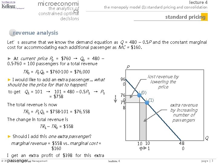
microeconomi the analytics of cs constrained optimal lecture 4 the monopoly model (I): standard pricing and consolidation standard pricing decisions revenue analysis Let’s assume that we know the demand equation as Q = 480 – 0. 5 P and the constant marginal cost for accommodating each additional passenger as MC = $160. ► At current price P 0 = $760 → Q 0 = 480 – 0. 5∙ 760 = 100 passengers for a total revenue P TR 0 = P 0 Q 0 = $760∙ 100 = $76, 000 lost revenue by lowering the price 96 0 ► I would like to add an extra passenger… what should be the price for that to happen? to get Q 1 = 101 → 101 = 480 – 0. 5 P 1 → P 1 = $758 76 0 75 8 The total revenue is now TR 1 = P 1 Q 1 = $758∙ 101 = $76, 558 (0) (1) The change in total revenue is extra revenue by increasing number of passengers TR 1 – TR 0 = $558 ► Should I add this one extra passenger? marginal revenue = $558 vs. marginal cost = 10 10 0 1 $160 I get an extra profit of $398 for this extra 2016 Kellogg School of Management passenger… lecture 4 48 0 Q page | 3

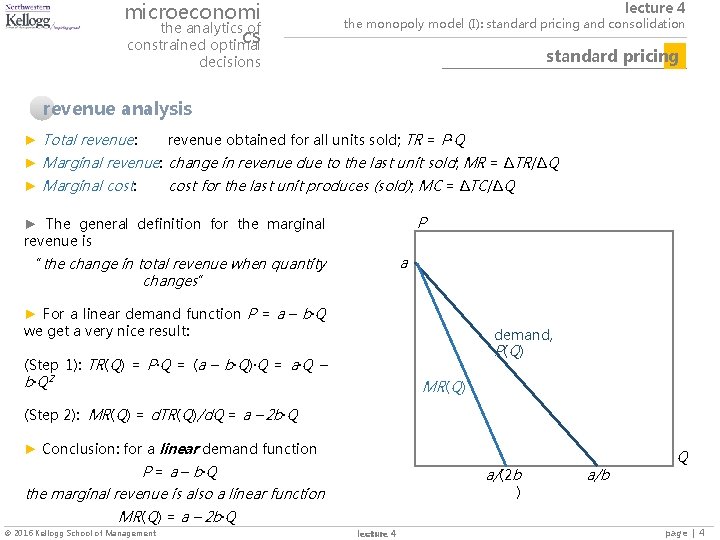
microeconomi the analytics of cs constrained optimal lecture 4 the monopoly model (I): standard pricing and consolidation standard pricing decisions revenue analysis ► Total revenue: revenue obtained for all units sold; TR = P∙Q ► Marginal revenue: change in revenue due to the last unit sold; MR = ∆TR/∆Q ► Marginal cost: cost for the last unit produces (sold); MC = ∆TC/∆Q P ► The general definition for the marginal revenue is a “the change in total revenue when quantity changes” ► For a linear demand function P = a – b∙Q we get a very nice result: demand, P(Q) (Step 1): TR(Q) = P∙Q = (a – b∙Q)∙Q = a∙Q – b∙Q 2 MR(Q) (Step 2): MR(Q) = d. TR(Q)/d. Q = a – 2 b∙Q ► Conclusion: for a linear demand function P = a – b∙Q a/(2 b ) the marginal revenue is also a linear function a/b Q MR(Q) = a – 2 b∙Q 2016 Kellogg School of Management lecture 4 page | 4

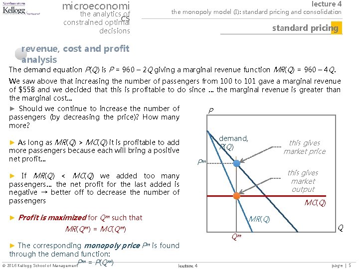
microeconomi the analytics of cs constrained optimal lecture 4 the monopoly model (I): standard pricing and consolidation standard pricing decisions revenue, cost and profit analysis The demand equation P(Q) is P = 960 – 2 Q giving a marginal revenue function MR(Q) = 960 – 4 Q. We saw above that increasing the number of passengers from 100 to 101 gave a marginal revenue of $558 and we decided that this is profitable to do since … the marginal revenue is greater than the marginal cost… ► Should we continue to increase the number of passengers (by decreasing the price)? How many more? ► As long as MR(Q) > MC(Q) it is profitable to add more passengers because each will bring a positive net profit… P demand, P(Q) this gives market price Pm this gives market output ► If MR(Q) < MC(Q) we added too many passengers… the net profit for the last added is negative → better off to decrease the number of passengers MC(Q) ► Profit is maximized for Qm such that MR(Qm) = MC(Qm) ► The corresponding monopoly price Pm is found through the demand function: m = P(Qm) 2016 Kellogg School of Management. P lecture 4 MR(Q) Qm Q page | 5

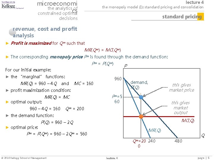
microeconomi the analytics of cs constrained optimal lecture 4 the monopoly model (I): standard pricing and consolidation standard pricing decisions revenue, cost and profit analysis ► Profit is maximized for Qm such that MR(Qm) = MC(Qm) ► The corresponding monopoly price Pm is found through the demand function: Pm = P(Qm) P For our initial example: ► the “marginal” functions: MR(Q) = 960 – 4 Q and MC = 160 960 ► profit maximization condition: ► optimal output: MR(Q) = MC 960 – 4 Q = 160 demand, P(Q) this gives market price Pm=5 60 this gives market output Qm = 200 ► the demand function: ► optimal price: MC(Q) P(Q) = 960 – 2 Q MR(Q) Pm = P(Qm) = 960 – 2 Qm = 560 Qm=20 240 0 2016 Kellogg School of Management lecture 4 Q 480 page | 6

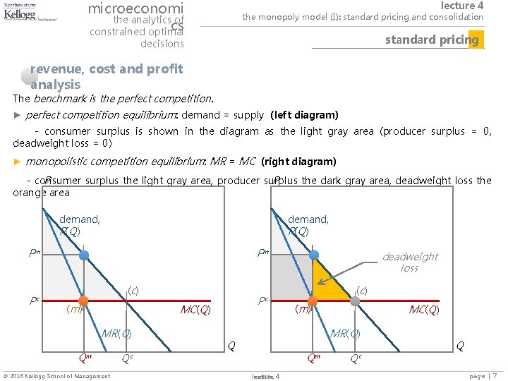
microeconomi the analytics of cs constrained optimal lecture 4 the monopoly model (I): standard pricing and consolidation standard pricing decisions revenue, cost and profit analysis The benchmark is the perfect competition. ► perfect competition equilibrium: demand = supply (left diagram) - consumer surplus is shown in the diagram as the light gray area (producer surplus = 0, deadweight loss = 0) ► monopolistic competition equilibrium: MR = MC (right diagram) P P - consumer surplus the light gray area, producer surplus the dark gray area, deadweight loss the orange area demand, P(Q) Pm Pc Pm ( c) ( m) Pc MC(Q) MR(Q) Qm 2016 Kellogg School of Management Qc deadweight loss ( c) ( m) MC(Q) MR(Q) Q Qm lecture 4 Qc Q page | 7

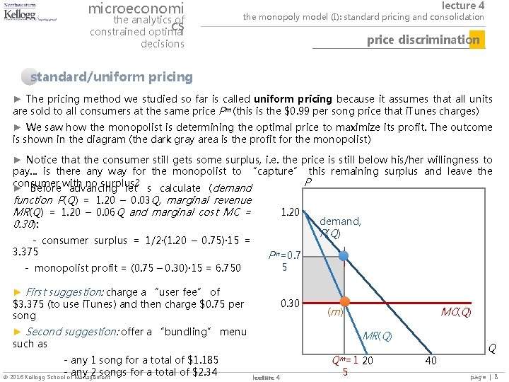
microeconomi the analytics of cs constrained optimal lecture 4 the monopoly model (I): standard pricing and consolidation price discrimination decisions standard/uniform pricing ► The pricing method we studied so far is called uniform pricing because it assumes that all units are sold to all consumers at the same price Pm (this is the $0. 99 per song price that i. Tunes charges) ► We saw how the monopolist is determining the optimal price to maximize its profit. The outcome is shown in the diagram (the dark gray area is the profit for the monopolist) ► Notice that the consumer still gets some surplus, i. e. the price is still below his/her willingness to pay… is there any way for the monopolist to “capture” this remaining surplus and leave the P consumer with no surplus? ► Before advancing let’s calculate (demand function P(Q) = 1. 20 – 0. 03 Q, marginal revenue 1. 20 MR(Q) = 1. 20 – 0. 06 Q and marginal cost MC = demand, 0. 30): P(Q) - consumer surplus = 1/2∙(1. 20 – 0. 75)∙ 15 = 3. 375 Pm=0. 7 5 - monopolist profit = (0. 75 – 0. 30)∙ 15 = 6. 750 ► First suggestion: charge a “user fee” of $3. 375 (to use i. Tunes) and then charge $0. 75 per song 0. 30 ( m) ► Second suggestion: offer a “bundling” menu such as - any 1 song for a total of $1. 185 - any 2 songs for a total of $2. 34 2016 Kellogg School of Management MC(Q) MR(Q) Qm=1 lecture 4 5 20 40 Q page | 8

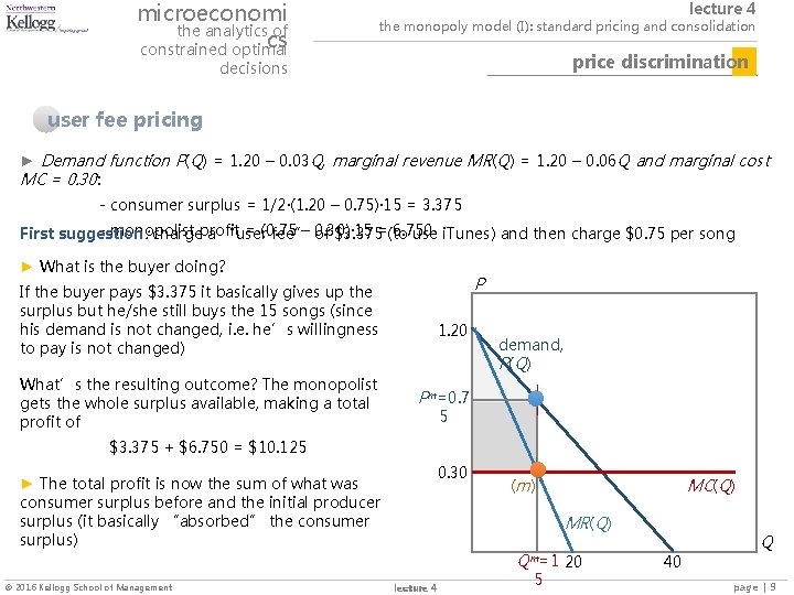
microeconomi the analytics of cs constrained optimal lecture 4 the monopoly model (I): standard pricing and consolidation price discrimination decisions user fee pricing ► Demand function P(Q) = 1. 20 – 0. 03 Q, marginal revenue MR(Q) = 1. 20 – 0. 06 Q and marginal cost MC = 0. 30: - consumer surplus = 1/2∙(1. 20 – 0. 75)∙ 15 = 3. 375 - monopolist = (0. 75 – 0. 30)∙ 15 6. 750 First suggestion : chargeprofit a “user fee” of $3. 375=(to use i. Tunes) and then charge $0. 75 per song ► What is the buyer doing? If the buyer pays $3. 375 it basically gives up the surplus but he/she still buys the 15 songs (since his demand is not changed, i. e. he’s willingness to pay is not changed) What’s the resulting outcome? The monopolist gets the whole surplus available, making a total profit of P 1. 20 demand, P(Q) Pm=0. 7 5 $3. 375 + $6. 750 = $10. 125 ► The total profit is now the sum of what was consumer surplus before and the initial producer surplus (it basically “absorbed” the consumer surplus) 0. 30 ( m) MR(Q) Qm=1 2016 Kellogg School of Management MC(Q) lecture 4 5 20 40 Q page | 9

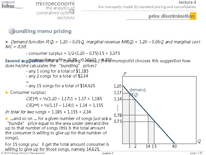
microeconomi the analytics of cs constrained optimal lecture 4 the monopoly model (I): standard pricing and consolidation price discrimination decisions bundling menu pricing ► Demand function P(Q) = 1. 20 – 0. 03 Q, marginal revenue MR(Q) = 1. 20 – 0. 06 Q and marginal cost MC = 0. 30: - consumer surplus = 1/2∙(1. 20 – 0. 75)∙ 15 = 3. 375 - monopolist profit = (0. 75 – 0. 30)∙ 15 = If 6. 750 Second suggestion : offer a “bundling” menu… the monopolist chooses this suggestion how does he/she calculates the “bundling” prices? - any 1 song for a total of $1. 185 P - any 2 songs for a total of $2. 34 … - any 15 songs for a total of $14. 625 1. 20 demand, ► Consumer surplus: 1. 17 P(Q) st CS(1 ) = ½(1. 20 – 1. 17)1 + 1. 17 = 1. 185 1. 14 CS(2 nd) = ½(1. 17 – 1. 14)1 + 1. 14 = 1. 155 In total for two songs = 1. 185 + 1. 155 = 2. 34 0. 78 ► …and so on … for a given number of songs just ask a “bundle” price equal to the area under demand line 0. 75 up to that number of songs (this is the total amount the consumer is willing to give up for that number of songs). For 15 songs you’ll get the total amount consumer is willing to give up for those songs, namely 14. 625. 2016 Kellogg School of Management lecture 4 1 2 14 15 40 Q page | 10

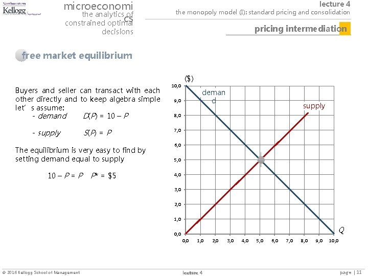
microeconomi the analytics of cs constrained optimal lecture 4 the monopoly model (I): standard pricing and consolidation pricing intermediation decisions free market equilibrium Buyers and seller can transact with each other directly and to keep algebra simple let’s assume: - demand D(P) = 10 – P - supply S( P ) = P The equilibrium is very easy to find by setting demand equal to supply 10 – P = P P* = $5 10, 0 ($) deman d 9, 0 supply 8, 0 7, 0 6, 0 5, 0 4, 0 3, 0 2, 0 1, 0 Q 0, 0 2016 Kellogg School of Management 1, 0 lecture 4 2, 0 3, 0 4, 0 5, 0 6, 0 7, 0 8, 0 9, 0 10, 0 page | 11

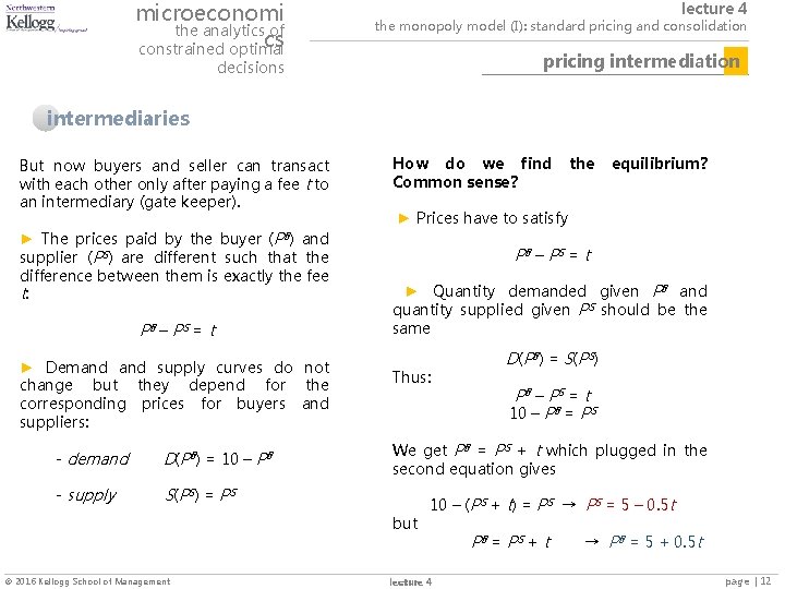
microeconomi the analytics of cs constrained optimal lecture 4 the monopoly model (I): standard pricing and consolidation pricing intermediation decisions intermediaries But now buyers and seller can transact with each other only after paying a fee t to an intermediary (gate keeper). (PB) ► The prices paid by the buyer and supplier (PS) are different such that the difference between them is exactly the fee t: PB – PS = t ► Demand supply curves do not change but they depend for the corresponding prices for buyers and suppliers: - demand D(PB) = 10 – PB - supply S( P S ) = P S How do we find Common sense? equilibrium? ► Prices have to satisfy PB – PS = t ► Quantity demanded given PB and quantity supplied given PS should be the same Thus: D(PB) = S(PS) PB – PS = t 10 – PB = PS We get PB = PS + t which plugged in the second equation gives but 2016 Kellogg School of Management the 10 – (PS + t) = PS → PS = 5 – 0. 5 t lecture 4 PB = PS + t → PB = 5 + 0. 5 t page | 12

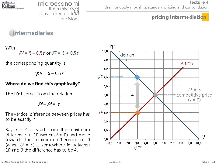
microeconomi the analytics of cs constrained optimal lecture 4 the monopoly model (I): standard pricing and consolidation pricing intermediation decisions intermediaries With 10, 0 PS = 5 – 0. 5 t or PB = 5 + 0. 5 t Where do we find this graphically? The hint comes from the relation PB – PS = t The vertical difference between prices has to be exactly t. Say t = 4 … start from the maximum difference of 10 (when Q = 0) and move towards the minimum difference of 0 (when Q = 5) … somewhere in between 10 and 0 the difference has to be 4. 2016 Kellogg School of Management deman d 9, 0 the corresponding quantity is Q(t) = 5 – 0. 5 t ($) supply 8, 0 PB 7, 0 6, 0 P* = 5 competitive price (t = 0) 4 5, 0 4, 0 PS 3, 0 2, 0 1, 0 Q 0, 0 1, 0 lecture 4 2, 0 3, 0 Q** 4, 0 5, 0 6, 0 7, 0 8, 0 9, 0 10, 0 page | 13

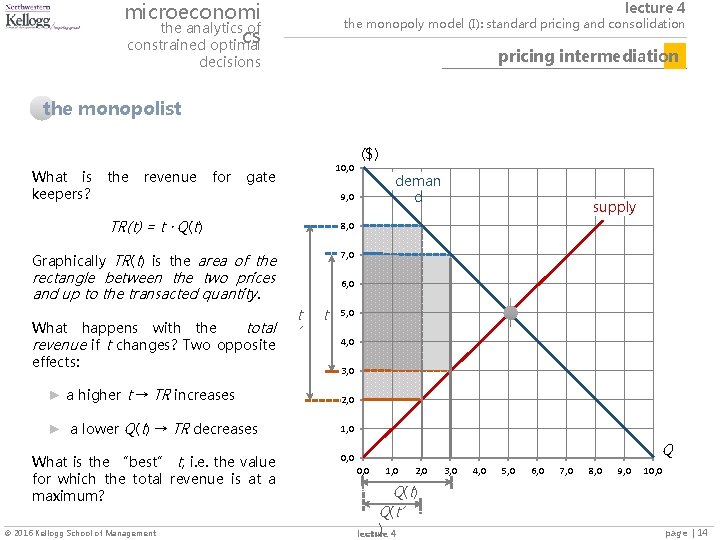
microeconomi the analytics of cs constrained optimal lecture 4 the monopoly model (I): standard pricing and consolidation pricing intermediation decisions the monopolist What is keepers? the revenue for 10, 0 gate ($) deman d 9, 0 TR(t) = t ∙ Q(t) 8, 0 Graphically TR(t) is the area of the 7, 0 rectangle between the two prices and up to the transacted quantity. What happens with the total revenue if t changes? Two opposite effects: 6, 0 t t ’ 5, 0 4, 0 3, 0 ► a higher t → TR increases 2, 0 ► a lower Q(t) → TR decreases 1, 0 What is the “best” t, i. e. the value for which the total revenue is at a maximum? 0, 0 2016 Kellogg School of Management supply Q 0, 0 1, 0 2, 0 3, 0 4, 0 5, 0 6, 0 7, 0 8, 0 9, 0 10, 0 Q ( t) Q(t’ ) 4 lecture page | 14

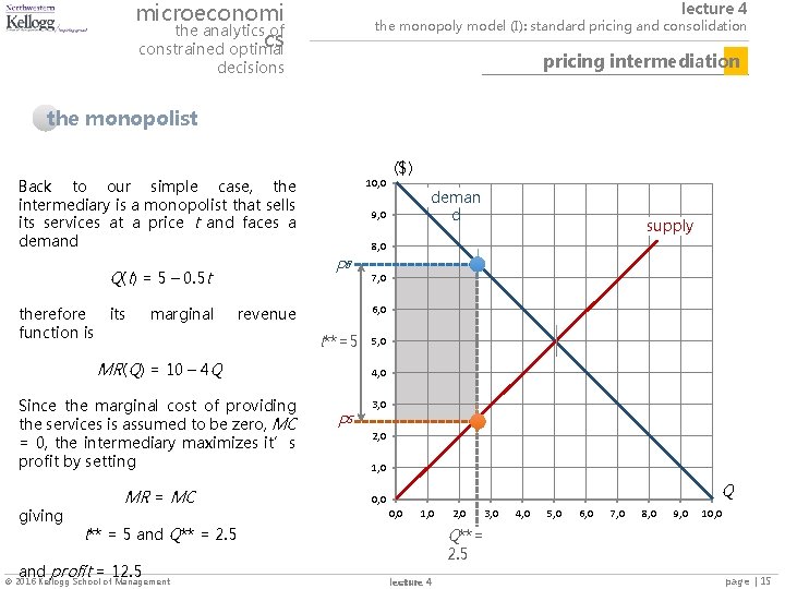
microeconomi the analytics of cs constrained optimal lecture 4 the monopoly model (I): standard pricing and consolidation pricing intermediation decisions the monopolist Back to our simple case, the intermediary is a monopolist that sells its services at a price t and faces a demand marginal giving 7, 0 t**=5 5, 0 4, 0 PS 3, 0 2, 0 1, 0 Q 0, 0 1, 0 t** = 5 and Q** = 2. 5 and profit = 12. 5 2016 Kellogg School of Management supply 6, 0 MR(Q) = 10 – 4 Q MR = MC deman d 8, 0 revenue Since the marginal cost of providing the services is assumed to be zero, MC = 0, the intermediary maximizes it’s profit by setting ($) 9, 0 PB Q(t) = 5 – 0. 5 t therefore its function is 10, 0 2, 0 3, 0 4, 0 5, 0 6, 0 7, 0 8, 0 9, 0 10, 0 Q**= 2. 5 lecture 4 page | 15

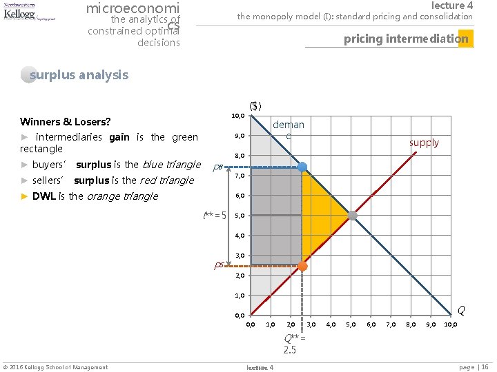
microeconomi the analytics of cs constrained optimal lecture 4 the monopoly model (I): standard pricing and consolidation pricing intermediation decisions surplus analysis 10, 0 Winners & Losers? ► intermediaries gain is the green rectangle ► buyers’ surplus is the blue triangle ► sellers’ surplus is the red triangle ($) deman d 9, 0 supply 8, 0 PB ► DWL is the orange triangle 7, 0 6, 0 t**=5 5, 0 4, 0 PS 3, 0 2, 0 1, 0 Q 0, 0 1, 0 2, 0 3, 0 4, 0 5, 0 6, 0 7, 0 8, 0 9, 0 10, 0 Q**= 2. 5 2016 Kellogg School of Management lecture 4 page | 16

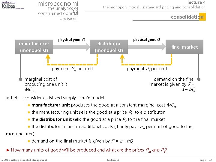
microeconomi the analytics of cs constrained optimal lecture 4 the monopoly model (I): standard pricing and consolidation decisions manufacturer (monopolist) physical good Q distributor (monopolist) payment Pm per unit final market payment Pd per unit marginal cost of producing one unit is demand on the final market is given by P = a – b. Q MCm ► Let’s consider a stylized supply –chain model: ● manufacturer unit produces the good at a constant marginal cost MCm ● the manufacturing unit sells the good at a price Pm to a distributor ● the distributor unit sells the good at a price Pd to the final market ● the distributor incurs no additional costs (it only pays Pm per unit of good to the manufacturer) ● demand on the final market is given by P = a – b. Q ► How many units of good will be produced and what are the prices Pm and Pd? 2016 Kellogg School of Management lecture 4 page | 17

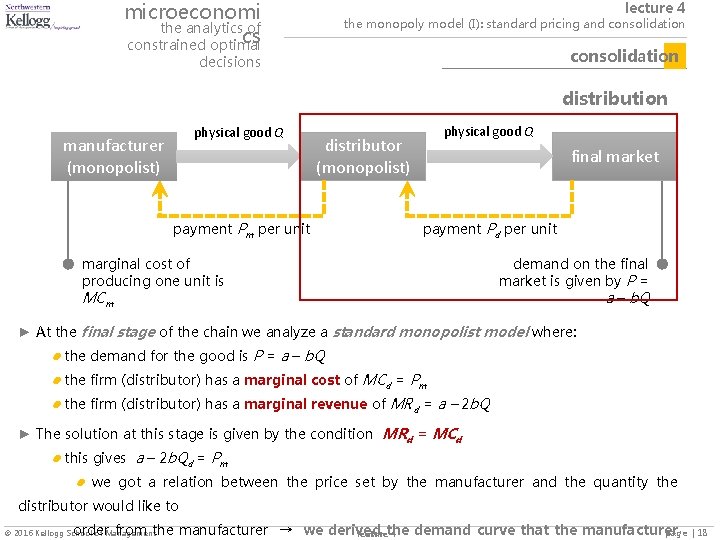
microeconomi the analytics of cs constrained optimal lecture 4 the monopoly model (I): standard pricing and consolidation decisions distribution physical good Q manufacturer (monopolist) physical good Q distributor (monopolist) payment Pm per unit final market payment Pd per unit marginal cost of producing one unit is MCm demand on the final market is given by P = a – b. Q ► At the final stage of the chain we analyze a standard monopolist model where: ● the demand for the good is P = a – b. Q ● the firm (distributor) has a marginal cost of MCd = Pm ● the firm (distributor) has a marginal revenue of MRd = a – 2 b. Q ► The solution at this stage is given by the condition MRd = MCd ● this gives a – 2 b. Qd = Pm ● we got a relation between the price set by the manufacturer and the quantity the distributor would like to order from the manufacturer → we derived demand curve that the manufacturer page lecturethe 4 2016 Kellogg School of Management | 18

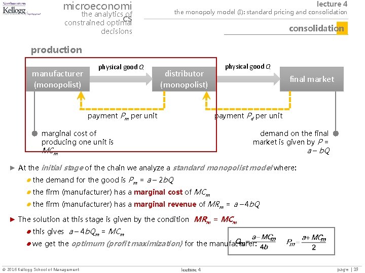
microeconomi the analytics of cs constrained optimal lecture 4 the monopoly model (I): standard pricing and consolidation decisions production manufacturer (monopolist) physical good Q distributor (monopolist) payment Pm per unit physical good Q final market payment Pd per unit marginal cost of producing one unit is demand on the final market is given by P = a – b. Q MCm ► At the initial stage of the chain we analyze a standard monopolist model where: ● the demand for the good is Pm = a – 2 b. Q ● the firm (manufacturer) has a marginal cost of MCm ● the firm (manufacturer) has a marginal revenue of MRm = a – 4 b. Q ► The solution at this stage is given by the condition MRm = MCm ● this gives a – 4 b. Qm = MCm ● we get the optimum (profit maximization) for the manufacturer: 2016 Kellogg School of Management lecture 4 page | 19

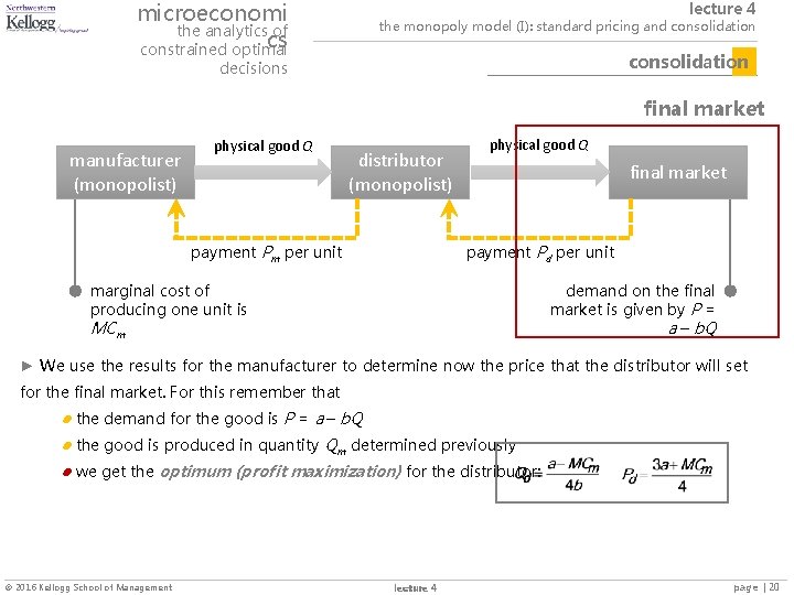
microeconomi the analytics of cs constrained optimal lecture 4 the monopoly model (I): standard pricing and consolidation decisions final market manufacturer (monopolist) physical good Q distributor (monopolist) payment Pm per unit physical good Q final market payment Pd per unit marginal cost of producing one unit is demand on the final market is given by P = a – b. Q MCm ► We use the results for the manufacturer to determine now the price that the distributor will set for the final market. For this remember that ● the demand for the good is P = a – b. Q ● the good is produced in quantity Qm determined previously ● we get the optimum (profit maximization) for the distributor: 2016 Kellogg School of Management lecture 4 page | 20

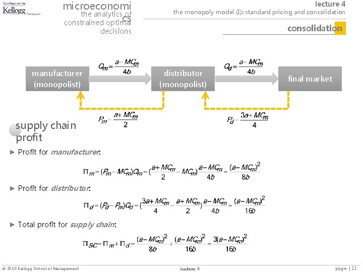
microeconomi the analytics of cs constrained optimal lecture 4 the monopoly model (I): standard pricing and consolidation decisions manufacturer (monopolist) distributor (monopolist) final market supply chain profit ► Profit for manufacturer: ► Profit for distributor: ► Total profit for supply chain: 2016 Kellogg School of Management lecture 4 page | 21

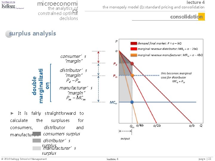
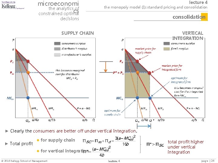
microeconomi the analytics of cs constrained optimal lecture 4 the monopoly model (I): standard pricing and consolidation decisions surplus analysis double marginalizati on consumer’s “margin” distributor’s “margin” Pd – P m manufacturer’s “margin” Pm – MCm ► It is fairly straightforward to calculate the consumers, manufacturer: surpluses distributor for and consumers surplus distributor’s surplus manufacturer’s surplus 2016 Kellogg School of Management lecture 4 page | 22

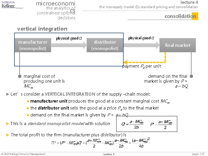
microeconomi the analytics of cs constrained optimal lecture 4 the monopoly model (I): standard pricing and consolidation decisions vertical integration manufacturer (monopolist) physical good Q distributor (monopolist) final market payment Pd per unit marginal cost of producing one unit is demand on the final market is given by P = a – b. Q MCm ► Let’s consider a VERTICAL INTEGRATION of the supply –chain model: ● manufacturer unit produces the good at a constant marginal cost MCm ● the distributor unit sells the good at a price Pd to the final market ● demand on the final market is given by P = a – b. Q ► This is a standard monopolist model with solution ► The total profit to the firm (manufacturer plus distributor) is 2016 Kellogg School of Management lecture 4 page | 23

microeconomi the analytics of cs constrained optimal lecture 4 the monopoly model (I): standard pricing and consolidation decisions VERTICAL INTEGRATION SUPPLY CHAIN ► Clearly the consumers are better off under vertical integration. ► Total profit ● for supply chain total profit higher under vertical integration ● for vertical integration 2016 Kellogg School of Management lecture 4 page | 24