session the perfectly competitive market three demand supply

microeconomi the analytics of cs constrained optimal lecture 3 the perfectly competitive market &

microeconomi the analytics of cs constrained optimal ► Tax on consumers lecture 3 the

Slides: 19

Download presentation

session the perfectly competitive market three demand supply curves …………. revisited 1 market mechanism and …………. 2 equilibrium market dynamics: shifting …………. 3 market dynamics: curves long- …………. 5 run …………. market dynamics: key points …………. 8 consumer surplus 9 producer surplus ……… 11 market efficiency analysis ………. 1 3 price floor analysis ……… 14 price ceiling analysis ………. 1 5 consumer tax analysis ………. 1 6 tax incidence analysis ……… 17 key points ………. 1 8 spring 2016 microeco the analytics of nomics constrained

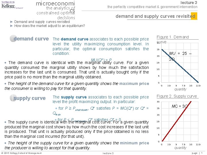
microeconomi the analytics of cs constrained optimal lecture 3 the perfectly competitive market & government intervention demand supply curves revisited decisions ► Demand supply curves revisited ► How does the market adjust to an equilibrium? demand curve The demand curve associates to each possible price level the utility maximizing consumption level. In particular, the optimal consumption satisfies the condition: MU(Q*) = P The demand curve is identical with the marginal utility curve. For a given quantity consumed the marginal utility shows by how much the satisfaction increases for the last unit is consumed. That unit is actually bought only if the price paid is no more than the marginal utility obtained. The height of the demand curve for a given quantity shows the maximum price the consumer is willing to pay for that quantity. supply curve 25 MU = 25 – 2 Q 20 15 10 5 0 0 2. 5 5 7. 5 quantity 10 12. 5 The supply curve associates to each possible price level the profit maximizing output. In particular: Figure 2. Supply curve for P Pshut-down, Q* satisfies P = MC(Q*) or Q* = Qmax 25 for P < P , Q* satisfies Q* = 0 The supply curve is identical with theshut-down marginal cost curve. For a given quantity produced the marginal cost shows by how much the cost increases if the last unit is produced. That unit is actually produced only if the price obtained is no less than the marginal cost incurred (for that unit). The height of the supply curve for a given quantity shows the minimum price the producer is willing to accept for that quantity. 2016 Kellogg School of Management Figure 1. Demand curve 30 lecture 3 30 MC = 3 Q 20 15 10 5 0 0 2. 5 5 7. 5 quantity 10 12. 5 page | 1

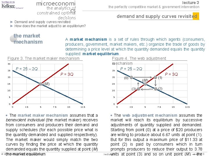
microeconomi the analytics of cs constrained optimal lecture 3 the perfectly competitive market & government intervention demand supply curves revisited decisions ► Demand supply curves revisited ► How does the market adjust to an equilibrium? the market mechanism A market mechanism is a set of rules through which agents (consumers, producers, government, market makers, etc. ) organize the trade of goods by determining a price level at which the quantity demanded equals the quantity supplied: market equilibrium. Figure 3. The market maker mechanism Figure 4. The web adjustment mechanism 30 30 P = 25 – 2 Q 25 25 P = 3 Q 20 20 (M) 15 10 5 5 0 2. 5 5 (M) 15 10 0 (0) 7. 5 10 12. 5 The market maker mechanism assumes that a benevolent individual (the market maker) receives from consumers and producers their demand supply schedules (for each possible price what is the quantity demanded and supplied respectively). The market maker would simply match the two curves by finding the price at which the quantity demanded equals the quantity supplied at point (M) 2016 School of Management the. Kellogg market equilibrium 0 (2) (3) 0 2. 5 (1) 5 7. 5 10 12. 5 The web adjustment mechanism assumes the market will reach its equilibrium by successive adjustments of quantity supplied and demanded. Starting from point (0) at a price of $20 producers are willing to produce about 6. 67 units at point (1). But for this output a maximum price of $11. 33 at point (2) is paid by consumers which in turn prompts producers to reduce their output to 3. 78 lecture 3 units at point (3) and so on unit point (M) –page the| 2

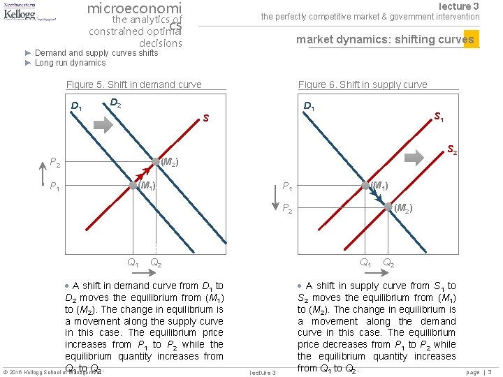
microeconomi the analytics of cs constrained optimal lecture 3 the perfectly competitive market & government intervention market dynamics: shifting curves decisions ► Demand supply curves shifts ► Long run dynamics Figure 5. Shift in demand curve D 1 Figure 6. Shift in supply curve D 2 D 1 S (M 2) P 2 P 1 S 2 (M 1) P 1 (M 1) (M 2) P 2 Q 1 Q 2 A shift in demand curve from D 1 to D 2 moves the equilibrium from (M 1) to (M 2). The change in equilibrium is a movement along the supply curve in this case. The equilibrium price increases from P 1 to P 2 while the equilibrium quantity increases from 1 to Q 2. 2016 Kellogg School of. Q Management Q 1 lecture 3 Q 2 A shift in supply curve from S 1 to S 2 moves the equilibrium from (M 1) to (M 2). The change in equilibrium is a movement along the demand curve in this case. The equilibrium price decreases from P 1 to P 2 while the equilibrium quantity increases from Q 1 to Q 2. page | 3

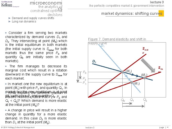
microeconomi the analytics of cs constrained optimal lecture 3 the perfectly competitive market & government intervention market dynamics: shifting curves decisions ► Demand supply curves shifts ► Long run dynamics Consider a firm serving two markets characterized by demand curves D 1 and D 2. They intersecting at point (M 0) which is the initial equilibrium in both markets (the initial supply curve is Sinitial for both markets thus the same price P 0 and quantity Q 0 are initially seen in both markets). The firm manages to decrease its marginal cost which result in a rotation downward in the supply curve to Snew for each market. In market one the new equilibrium is at point (M 1) with price P 1 and quantity Q 1. In the new is at point market What two explains theequilibrium different reaction in (M ) with price P and quantity Q. 2 P 2 and the 2 two markets 2(notice that P 1 > Q 1 < Q 2)? Which demand is more elastic at the initial point (M 0)? Figure 7. Demand elasticity and shift in supply curve D 1 Siniti al D 2 Sne (M 0) P 0 P 2 P 1 (M 2) w (M 1) Q 0 Q 1 Q 2 A change in price will result in a higher change in quantity for a more elastic demand. In this case D 2 is more elastic than D 1 at the initial point (M 0). 2016 Kellogg School of Management lecture 3 page | 4

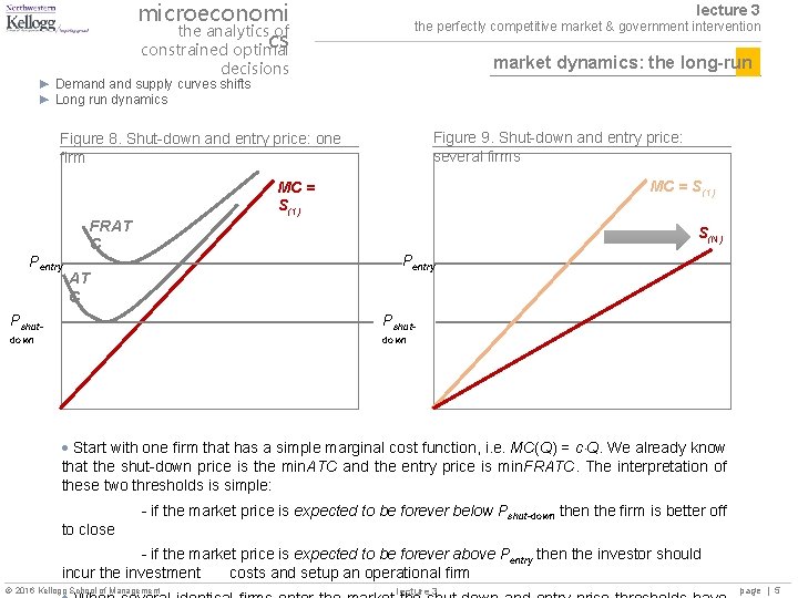
microeconomi the analytics of cs constrained optimal lecture 3 the perfectly competitive market & government intervention market dynamics: the long-run decisions ► Demand supply curves shifts ► Long run dynamics Figure 9. Shut-down and entry price: several firms Figure 8. Shut-down and entry price: one firm MC = S(1) Pentry FRAT C S(N) Pentry AT C Pshut- down Start with one firm that has a simple marginal cost function, i. e. MC(Q) = c Q. We already know that the shut-down price is the min. ATC and the entry price is min. FRATC. The interpretation of these two thresholds is simple: to close - if the market price is expected to be forever below Pshut-down the firm is better off - if the market price is expected to be forever above Pentry then the investor should incur the investment costs and setup an operational firm 2016 Kellogg School of Management lecture 3 page | 5

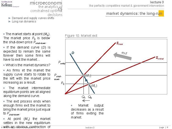
microeconomi the analytics of cs constrained optimal lecture 3 the perfectly competitive market & government intervention market dynamics: the long-run decisions ► Demand supply curves shifts ► Long run dynamics The market starts at point (M 0). The market price P 0 is below the shut-down price Pshut-down. If the demand curve (D) is expected to remain the same forever then some firms will have to exit the market… What is the market dynamics? As firms et the market the supply curve starts to rotate to the left with the market price increasing as a result. The market intermediate equilibrium points are all aligned along the demand curve. The exit process ends when enough firms exit the market to bring the market price just equal to Pshut-down. At point (M 1) the market settles in the new equilibrium 2016 of Management with. Kellogg an School obvious contraction of Figure 10. Market exit Snew exit D Sinitial Pentry Pshut- (M 1) down P 0 (M 0) Q 1 Q 0 Market output decreases as a result of firms exiting the market. lecture 3 page | 6

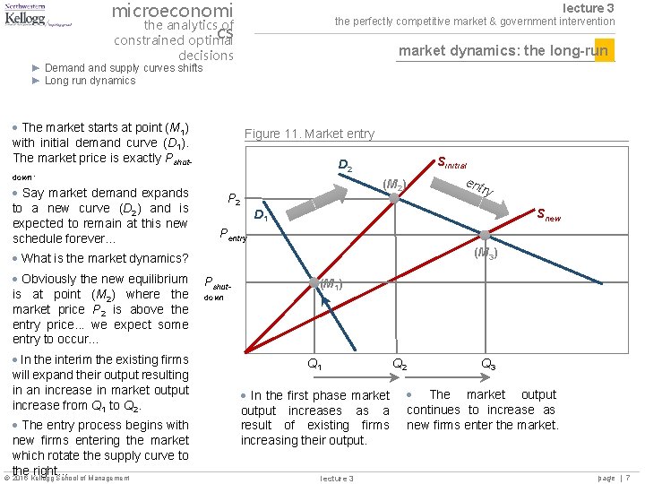
microeconomi the analytics of cs constrained optimal lecture 3 the perfectly competitive market & government intervention market dynamics: the long-run decisions ► Demand supply curves shifts ► Long run dynamics The market starts at point (M 1) with initial demand curve (D 1). The market price is exactly Pshutdown. Say market demand expands to a new curve (D 2) and is expected to remain at this new schedule forever… Figure 11. Market entry Sinitial D 2 P 2 (M 2) In the interim the existing firms will expand their output resulting in an increase in market output increase from Q 1 to Q 2. The entry process begins with new firms entering the market which rotate the supply curve to the right… 2016 Kellogg School of Management ry Snew D 1 Pentry (M 3) What is the market dynamics? Obviously the new equilibrium is at point (M 2) where the market price P 2 is above the entry price. . . we expect some entry to occur… ent Pshut- (M 1) down Q 1 In the first phase market output increases as a result of existing firms increasing their output. lecture 3 Q 2 Q 3 The market output continues to increase as new firms enter the market. page | 7

microeconomi the analytics of cs constrained optimal lecture 3 the perfectly competitive market & government intervention market dynamics: key points decisions ► Demand supply curves shifts ► Long run dynamics ► The market equilibrium will be found at the intersection of demand supply curves… ► We can distinguish the short-run dynamics and the long-run dynamics: - the short-run refers to the adjustment from a current equilibrium to the new equilibrium through an adjustment of output for existing firms - the long-run refers to the adjustment from a current equilibrium to the new equilibrium through an adjustment in the number of firms operating in the market (exit or entry) ► The critical point in understanding the long-run adjustment is always to consider the shut-down and entry threshold prices in relation to a “hypothetical” forever price level… 2016 Kellogg School of Management lecture 3 page | 8

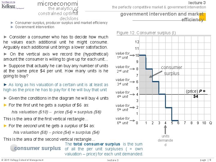
microeconomi the analytics of cs constrained optimal lecture 3 the perfectly competitive market & government intervention and market efficiency decisions ► Consumer surplus, producer surplus and market efficiency ► Government intervention ► Consider a consumer who has to decide how much he values each additional unit he might consume. Arguably each additional unit brings a lower satisfaction. Figure 12. Consumer surplus (I) 12 11 ► On the vertical axis we record the (hypothetical) amount the consumer is willing to give up for each unit… value for 1 st unit ► Suppose that actually he can buy any number of units at the same price $4 per unit. How many units is he going to buy? value for 2 nd unit ► As long as his valuation of a certain unit is at least as high as the price he has to pay for it he will buy that unit ► Given the conditions in the diagram he will buy 4 units ► For the first unit he gets a surplus of $6 as: his valuation ($10) – price ($4) = surplus ($6) This is the area of the first vertical rectangle… ► For the second unit he gets a surplus of $4 as: 10 9 7 value for 3 rd unit 6 5 value for 4 th unit (price) P = $4 4 3 value for 5 th unit value for 6 th unit 2 1 0 his valuation ($8) – price ($4) = surplus ($4) This is the area of the second vertical rectangle… The total consumer surplus is the sum consumer surplus of all the per unit surpluses ( = own valuation – price) for each unit demanded. 2016 Kellogg School of Management consumer surplus 8 lecture 3 1 2 3 4 5 6 7 8 9 10 Q units demande d page | 9

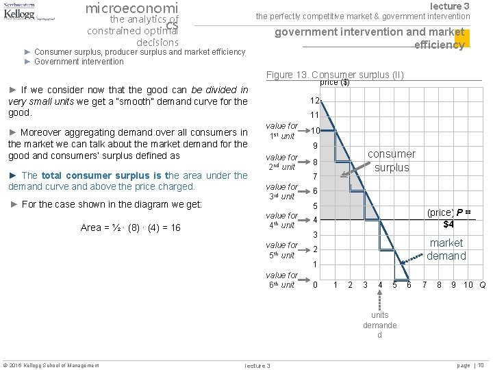
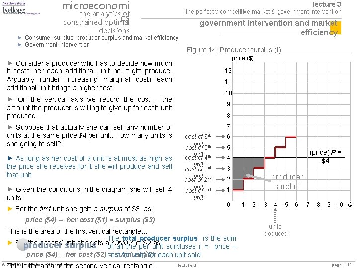
microeconomi the analytics of cs constrained optimal lecture 3 the perfectly competitive market & government intervention and market efficiency decisions ► Consumer surplus, producer surplus and market efficiency ► Government intervention Figure 14. Producer surplus (I) price ($) ► Consider a producer who has to decide how much it costs her each additional unit he might produce. Arguably (under increasing marginal cost) each additional unit brings a higher cost. 12 11 10 ► On the vertical axis we record the cost – the amount the producer is willing to give up for each unit produced… ► Suppose that actually she can sell any number of units at the same price $4 per unit. How many units is she going to sell? ► As long as her cost of a unit is at most as high as the price she receives for it she will produce and sell that unit ► Given the conditions in the diagram she will sell 4 units 9 8 7 cost of 6 th unit cost of 5 th costunit of 4 th unit cost of 3 rd unit cost of 2 nd unit cost of 1 st unit 6 5 3 1 price ($4) – her cost ($1) = surplus ($3) This is the area of the first vertical rectangle… The total producer surplus is the sum ► Forproducer the second unit she gets a surplus of $2 as: surplus of all the per unit surpluses ( = price – price ($4) – her cost ($2) cost = surplus ($2) for unit) for each unit sold. This is the area of the second vertical rectangle… 2016 Kellogg School of Management lecture 3 producer surplus 2 0 ► For the first unit she gets a surplus of $3 as: (price) P = $4 4 1 2 3 4 5 6 7 8 9 10 Q units produced page | 11

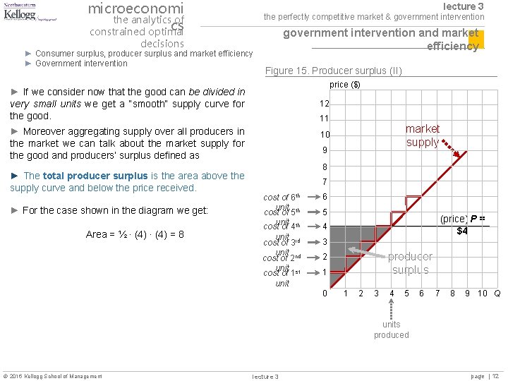
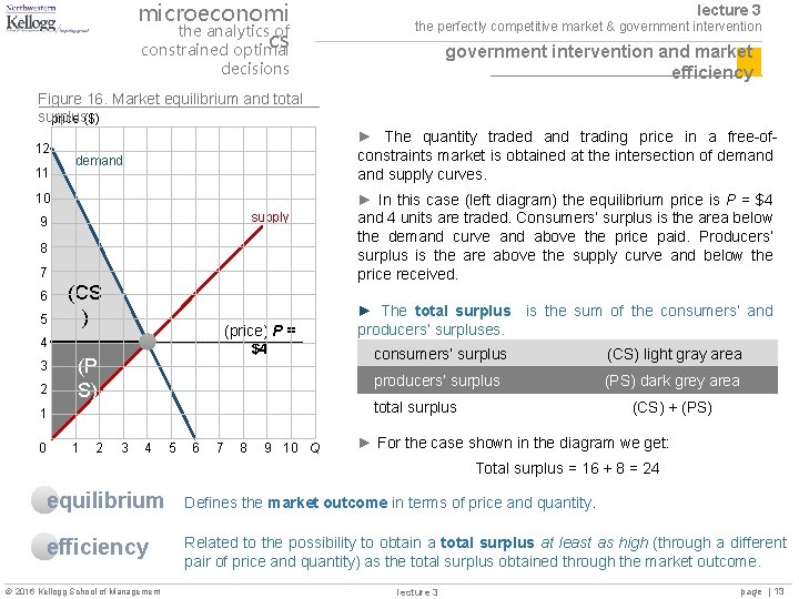
microeconomi the analytics of cs constrained optimal lecture 3 the perfectly competitive market & government intervention and market efficiency decisions Figure 16. Market equilibrium and total surplus price ($) 12 11 ► The quantity traded and trading price in a free-ofconstraints market is obtained at the intersection of demand supply curves. demand 10 supply 9 8 7 6 5 (CS ) (price) P = $4 4 3 2 (P S) 1 2 ► The total surplus is the sum of the consumers’ and producers’ surpluses. consumers’ surplus (CS) light gray area producers’ surplus (PS) dark grey area total surplus 1 0 ► In this case (left diagram) the equilibrium price is P = $4 and 4 units are traded. Consumers’ surplus is the area below the demand curve and above the price paid. Producers’ surplus is the are above the supply curve and below the price received. 3 4 5 6 7 8 9 10 Q (CS) + (PS) ► For the case shown in the diagram we get: Total surplus = 16 + 8 = 24 equilibrium Defines the market outcome in terms of price and quantity. efficiency Related to the possibility to obtain a total surplus at least as high (through a different pair of price and quantity) as the total surplus obtained through the market outcome. 2016 Kellogg School of Management lecture 3 page | 13

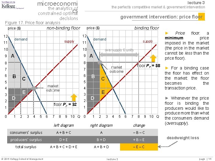
microeconomi the analytics of cs constrained optimal lecture 3 the perfectly competitive market & government intervention: price floor decisions Figure 17. Price floor analysis non-binding floor price ($) 12 11 12 demand supply A 9 8 8 7 7 6 B 4 2 6 C 5 3 E D floor PF = $2 1 2 3 4 5 6 7 8 A 2 floor PF = $8 market outcome B C 4 3 supply oversupply 6 units 5 market outcome 1 0 demand 11 10 10 9 binding floor price ($) E D 1 9 10 Q 0 1 2 3 4 5 6 7 8 9 10 Q left diagram right diagram change consumers’ surplus A+B+C A –B–C producers’ surplus D+E B+D +B–E total surplus A+B+C+D+E A+B+D –E–C 2016 Kellogg School of Management lecture 3 ► Price floor: a minimum price imposed in the market (the price in the market cannot be less than the price floor). ► For a binding case the floor has effect on the market: the floor becomes the transaction price. ► Whenever the price floor is binding the producers would like to produce more than what the consumers demand (oversupply). deadweight loss page | 14

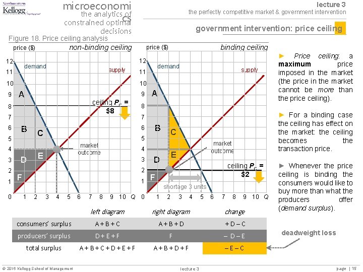
microeconomi the analytics of cs constrained optimal lecture 3 the perfectly competitive market & government intervention: price ceiling decisions Figure 18. Price ceiling analysis non-binding ceiling price ($) 12 12 demand 11 supply A 9 ceiling PC = $8 8 7 6 B 4 2 1 0 supply 3 2 1 1 2 3 4 5 6 7 8 B C 4 F ► For a binding case the ceiling has effect on the market: the ceiling becomes the transaction price. 7 5 market outcome E D A 9 10 Q 0 market outcome E D ceiling PC = $2 F shortage 3 units 1 2 3 4 5 6 7 8 9 10 Q left diagram right diagram change consumers’ surplus A+B+C A+B+D +D–C producers’ surplus D+E+F F – D–E total surplus A+B+C+D+E+F A+B+D+F –E–C 2016 Kellogg School of Management ► Price ceiling: a maximum price imposed in the market (the price in the market cannot be more than the price ceiling). 8 6 C 5 3 demand 11 10 10 9 binding ceiling price ($) lecture 3 ► Whenever the price ceiling is binding the consumers would like to buy more than what the producers offer (demand surplus). deadweight loss page | 15

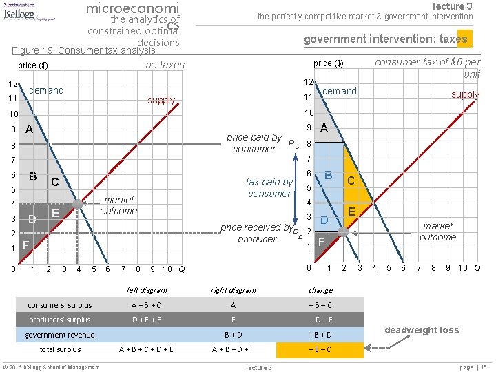
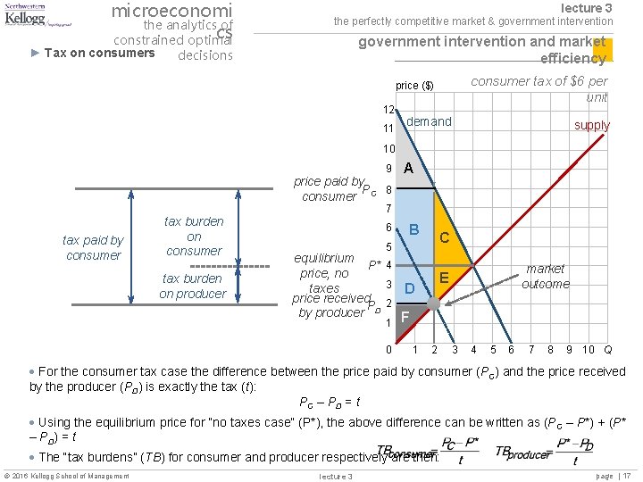
microeconomi the analytics of cs constrained optimal lecture 3 the perfectly competitive market & government intervention: taxes decisions Figure 19. Consumer tax analysis no taxes price ($) 12 11 12 demand 11 supply A 9 price paid by PC 8 consumer 8 B C 5 4 3 market outcome E D tax paid by consumer 0 A B C 5 4 E D market outcome price received by 2 PD producer 1 F F 1 6 3 2 1 supply 7 7 6 demand 10 10 9 consumer tax of $6 per unit price ($) 2 3 4 5 6 7 8 0 9 10 Q 1 left diagram right diagram change consumers’ surplus A+B+C A –B–C producers’ surplus D+E+F F –D–E B+D +B+D A+B+D+F –E–C government revenue total surplus 2016 Kellogg School of Management A+B+C+D+E lecture 3 2 3 4 5 6 7 8 9 10 Q deadweight loss page | 16

microeconomi the analytics of cs constrained optimal ► Tax on consumers lecture 3 the perfectly competitive market & government intervention and market efficiency decisions consumer tax of $6 per unit price ($) 12 11 demand supply 10 9 price paid by P 8 consumer C tax paid by consumer tax burden on producer A 7 6 B C 5 equilibrium P* 4 price, no 3 D taxes price received 2 P by producer D F market outcome E 1 0 1 2 3 4 5 6 7 8 9 10 Q For the consumer tax case the difference between the price paid by consumer (PC) and the price received by the producer (PD) is exactly the tax (t): PC – PD = t Using the equilibrium price for “no taxes case” (P*), the above difference can be written as (PC – P*) + (P* – PD) = t The “tax burdens” (TB) for consumer and producer respectively are then: 2016 Kellogg School of Management lecture 3 page | 17

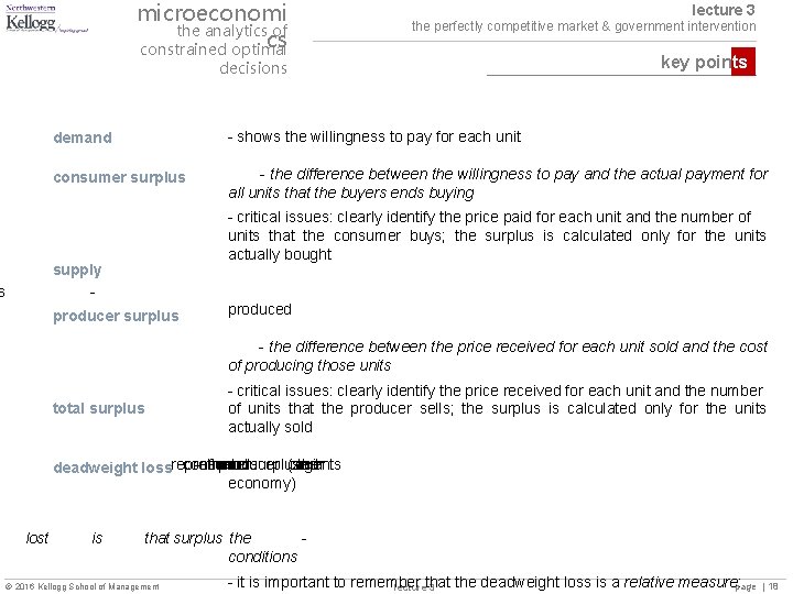
microeconomi the analytics of cs constrained optimal lecture 3 the perfectly competitive market & government intervention decisions ► DEMAND: demand key points - shows the willingness to pay for each unit ► CONSUMER consumer surplus. SURPLUS: - the difference between the willingness to pay and the actual payment for all units that the buyers ends buying supply ► SUPPLY: - s producer surplus - critical issues: clearly identify the price paid for each unit and the number of units that the consumer buys; the surplus is calculated only for the units actually bought produced ► PRODUCER SURPLUS: - the difference between the price received for each unit sold and the cost of producing those units total surplus - critical issues: clearly identify the price received for each unit and the number of units that the producer sells; the surplus is calculated only for the units actually sold ► APPLICATIONS: consumer -sum ofthe producer and surpluses (and other agents in deadweight lossrepresent economy) lost ► DEADWEIGHT is that surplus LOSS: the conditions 2016 Kellogg School of Management - it is important to remember the deadweight loss is a relative measure: page lecturethat 3 | 18